Laplace’s transform: from functions of t to functions of s

Laplace’s integral F(s) = int_0^inf f(t) e^{-st} dt turns differentiation into multiplication by s. This example computes the transform numerically for a few classical pairs, and uses the derivative rule to solve a damped oscillator algebraically.

import matplotlib.pyplot as plt
import numpy as np

from mathematicskit.special_functions import inverse_laplace_talbot, laplace_transform

Numerical transforms vs. the table

s = np.linspace(0.5, 5.0, 40)
pairs = {
    "exp(-t) -> 1/(s+1)": (lambda t: np.exp(-t), lambda s: 1 / (s + 1)),
    "t -> 1/s^2": (lambda t: t, lambda s: 1 / s**2),
    "sin(t) -> 1/(s^2+1)": (np.sin, lambda s: 1 / (s**2 + 1)),
}
fig, ax = plt.subplots()
for label, (f, F) in pairs.items():
    numeric = laplace_transform(f, s)
    print(f"{label:>22}: max error = {np.max(np.abs(numeric - F(s))):.1e}")
    ax.plot(s, F(s), label=label)
    ax.plot(s[::4], numeric[::4], "k.", ms=4)
ax.set_xlabel("s")
ax.set_ylabel("F(s)")
ax.set_yscale("log")
ax.set_title("Laplace transforms: quadrature (dots) vs. closed form")
ax.legend()

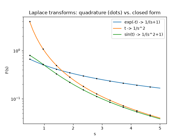
    exp(-t) -> 1/(s+1): max error = 1.2e-12
            t -> 1/s^2: max error = 2.6e-13
   sin(t) -> 1/(s^2+1): max error = 1.3e-11

<matplotlib.legend.Legend object at 0x7fd7c131e960>

Solving y’’ + 0.4 y’ + 4 y = 0, y(0) = 1, y’(0) = 0

L{y’} = sY - y(0) and L{y’’} = s^2 Y - s y(0) - y’(0), so Y(s) = (s + 0.4) / (s^2 + 0.4 s + 4): an algebraic equation in s.

def Y(s):
    return (s + 0.4) / (s**2 + 0.4 * s + 4.0)


# The poles -0.2 +- 1.99i must sit inside Talbot's contour, which needs
# t < m pi / (5 * 1.99); m = 40 covers t <= 10 with margin.

t = np.linspace(0.05, 10.0, 300)
omega = np.sqrt(4.0 - 0.04)
exact = np.exp(-0.2 * t) * (np.cos(omega * t) + 0.2 / omega * np.sin(omega * t))
y = inverse_laplace_talbot(Y, t, m=40)
print(f"max |y - exact| = {np.max(np.abs(y - exact)):.1e}")

fig, ax = plt.subplots()
ax.plot(t, exact, lw=3, alpha=0.4, label="closed form")
ax.plot(t, y, "--", label="inverse of Y(s)")
ax.set_xlabel("t")
ax.set_title("Damped oscillator solved in the s-domain")
ax.legend()

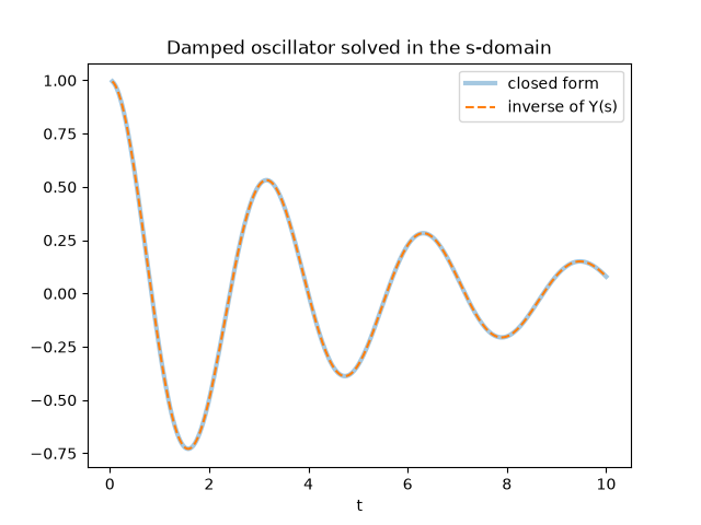
max |y - exact| = 7.3e-09

<matplotlib.legend.Legend object at 0x7fd7c19b0680>