Numerical Laplace inversion: Stehfest and Talbot

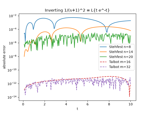
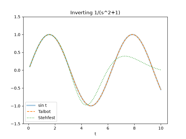
Stehfest’s 1970 algorithm inverts F(s) from real samples only, with alternating weights that cost digits to cancellation. Talbot’s 1979 contour winds the Bromwich integral around the negative real axis, where e^{st} decays, and reaches near machine precision, even for oscillating f(t) that Stehfest cannot resolve.

import matplotlib.pyplot as plt
import numpy as np

from mathematicskit.special_functions import inverse_laplace_stehfest, inverse_laplace_talbot, stehfest_coefficients

t = np.linspace(0.1, 10.0, 200)

The Stehfest weights grow like 10^(n/2)

for n in (6, 10, 14, 18):
    print(f"n={n:>2}: max |V_k| = {np.abs(stehfest_coefficients(n)).max():.2e}")

n= 6: max |V_k| = 8.58e+02
n=10: max |V_k| = 3.76e+05
n=14: max |V_k| = 1.70e+08
n=18: max |V_k| = 7.87e+10

A smooth function: both methods work

F = lambda s: 1.0 / (s + 1.0) ** 2  # t e^{-t}
exact = t * np.exp(-t)
fig, ax = plt.subplots()
for n in (8, 14, 20):
    ax.semilogy(t, np.abs(inverse_laplace_stehfest(F, t, n=n) - exact) + 1e-17, label=f"Stehfest n={n}")
for m in (16, 32):
    ax.semilogy(t, np.abs(inverse_laplace_talbot(F, t, m=m) - exact) + 1e-17, "--", label=f"Talbot m={m}")
ax.set_xlabel("t")
ax.set_ylabel("absolute error")
ax.set_title("Inverting 1/(s+1)^2 = L{t e^-t}")
ax.legend()

<matplotlib.legend.Legend object at 0x7fd7c64e2ab0>

An oscillating function: only Talbot succeeds

F = lambda s: 1.0 / (s**2 + 1.0)  # sin t
fig, ax = plt.subplots()
ax.plot(t, np.sin(t), lw=3, alpha=0.4, label="sin t")
ax.plot(t, inverse_laplace_talbot(F, t), "--", label="Talbot")
ax.plot(t, inverse_laplace_stehfest(F, t), ":", label="Stehfest")
ax.set_ylim(-1.5, 1.5)
ax.set_xlabel("t")
ax.set_title("Inverting 1/(s^2+1)")
ax.legend()

<matplotlib.legend.Legend object at 0x7fd7c2443710>