Haar’s wavelet: averages and differences at every scale

Haar’s 1910 orthonormal system of step functions splits a signal into a coarse average plus details at each scale: pairwise sums and differences over sqrt 2, repeated on the sums. A jump shows up as a single large coefficient per level, exactly where it happens.

import matplotlib.pyplot as plt
import numpy as np

from mathematicskit.special_functions import discrete_wavelet_transform, inverse_discrete_wavelet_transform
from mathematicskit.special_functions.visualizers.plots import plot_wavelet_decomposition

One level by hand

x = np.array([4.0, 2.0, 5.0, 5.0, 1.0, 3.0, 0.0, 0.0])
one = discrete_wavelet_transform(x, "haar", level=1)
print("pairwise sums / sqrt 2       :", np.round(one.approximation, 4))
print("pairwise differences / sqrt 2:", np.round(one.details[0], 4))

pairwise sums / sqrt 2       : [4.2426 7.0711 2.8284 0.    ]
pairwise differences / sqrt 2: [ 1.4142  0.     -1.4142  0.    ]

A piecewise-constant signal is sparse in the Haar basis

n = 256
signal = np.where(np.arange(n) < 100, 1.0, -0.5) + np.where((np.arange(n) >= 170) & (np.arange(n) < 200), 2.0, 0.0)
result = discrete_wavelet_transform(signal, "haar", level=5)
coefficients = np.concatenate([result.approximation, *result.details])
print(f"nonzero Haar coefficients: {np.sum(np.abs(coefficients) > 1e-12)} of {n}")
print(f"perfect reconstruction error: {np.max(np.abs(inverse_discrete_wavelet_transform(result) - signal)):.1e}")

fig, (ax0, ax1) = plt.subplots(2, 1, figsize=(8, 7))
ax0.step(np.arange(n), signal, where="post")
ax0.set_title("Piecewise-constant signal")
plot_wavelet_decomposition(result, ax=ax1)
fig.tight_layout()

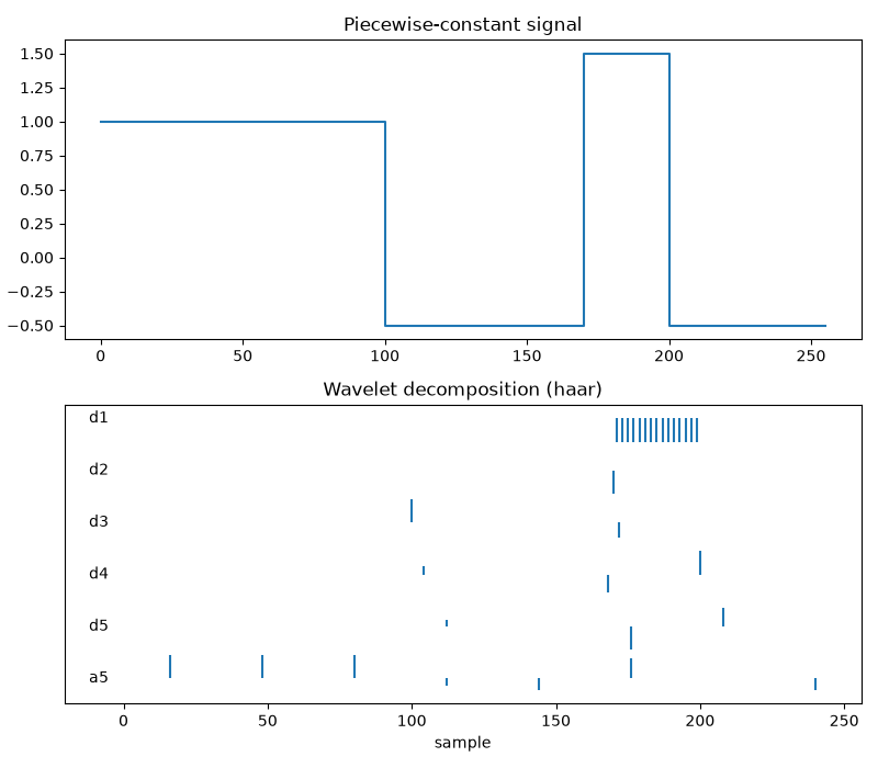
nonzero Haar coefficients: 16 of 256
perfect reconstruction error: 8.9e-16