Grossmann and Morlet’s continuous wavelet transform

Morlet, analysing seismic echoes, correlated the signal with shifted and dilated copies of a Gaussian-windowed complex exponential, and with Grossmann made the transform rigorous in 1984. The scalogram \(|W(s, t)|^2\) shows which frequencies are present when, which the Fourier transform alone cannot.

import matplotlib.pyplot as plt
import numpy as np

from mathematicskit.special_functions import morlet_cwt
from mathematicskit.special_functions.visualizers.plots import plot_scalogram

A chirp plus a short burst

dt = 0.002
t = np.arange(0.0, 4.0, dt)
chirp = np.sin(2 * np.pi * (5.0 * t + 5.0 * t**2))  # instantaneous frequency 5 + 10 t Hz
burst = np.exp(-(((t - 3.0) / 0.05) ** 2)) * np.sin(2 * np.pi * 80.0 * t)
x = chirp + burst

scales = np.geomspace(0.005, 0.4, 120)
result = morlet_cwt(x, scales, dt=dt)

fig, (ax0, ax1) = plt.subplots(2, 1, figsize=(8, 7), sharex=True)
ax0.plot(t, x, lw=0.6)
ax0.set_title("Chirp (5 -> 45 Hz) and an 80 Hz burst at t = 3 s")
plot_scalogram(result, ax=ax1)
ax1.plot(t, 5.0 + 10.0 * t, "w--", lw=1, label="chirp frequency 5 + 10t")
ax1.legend(loc="upper left")
fig.tight_layout()

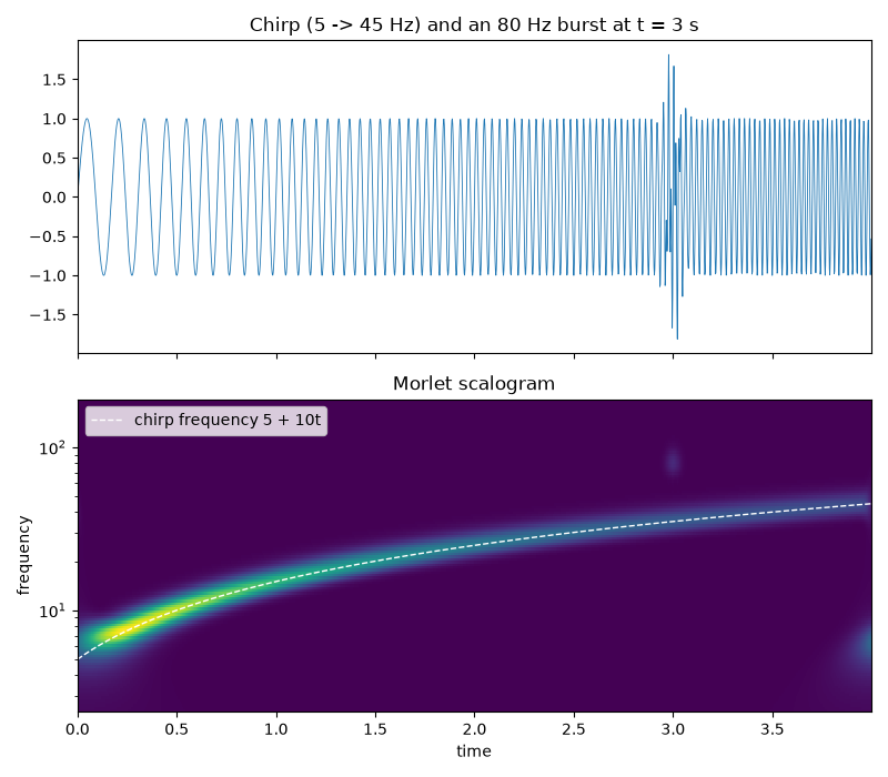
Ridge of the scalogram tracks the chirp

power = np.abs(result.coefficients) ** 2
chirp_band = result.frequencies < 60.0
for time in (0.5, 1.5, 2.5):
    col = int(time / dt)
    ridge = result.frequencies[chirp_band][np.argmax(power[chirp_band, col])]
    print(f"t = {time}: ridge at {ridge:5.1f} Hz (true {5 + 10 * time:.1f} Hz)")

t = 0.5: ridge at  10.2 Hz (true 10.0 Hz)
t = 1.5: ridge at  19.7 Hz (true 20.0 Hz)
t = 2.5: ridge at  29.6 Hz (true 30.0 Hz)