Benjamini-Hochberg and the false discovery rate

Runs 1000 one-sample t-tests, 100 of which have a real effect. With no correction, dozens of the “discoveries” are false; Bonferroni avoids false discoveries but misses most real effects; Benjamini-Hochberg keeps the fraction of false discoveries near the chosen 5% while finding far more of the real ones.

import matplotlib.pyplot as plt
import numpy as np

from mathematicskit.statistics import benjamini_hochberg, bonferroni_correction, one_sample_t_test

A thousand simultaneous tests

rng = np.random.default_rng(0)
m, m_real = 1000, 100
effect = np.zeros(m)
effect[:m_real] = 0.8
p_values = np.array([one_sample_t_test(rng.normal(loc=mu, size=20), mu0=0.0).p_value for mu in effect])
is_real = effect > 0

rejections = {
    "uncorrected": p_values <= 0.05,
    "Bonferroni": bonferroni_correction(p_values).rejected,
    "Benjamini-Hochberg": benjamini_hochberg(p_values).rejected,
}
for name, rejected in rejections.items():
    false = np.sum(rejected & ~is_real)
    true = np.sum(rejected & is_real)
    print(f"{name:19s}: {true:3d} true and {false:3d} false discoveries (FDP {false / max(true + false, 1):.3f})")

uncorrected        :  90 true and  46 false discoveries (FDP 0.338)
Bonferroni         :  10 true and   0 false discoveries (FDP 0.000)
Benjamini-Hochberg :  51 true and   4 false discoveries (FDP 0.073)

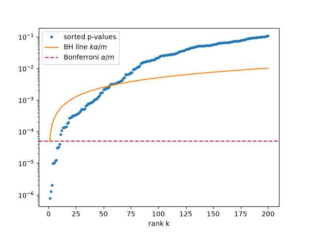
The step-up line

sorted_p = np.sort(p_values)[:200]
ranks = np.arange(1, sorted_p.size + 1)
fig, ax = plt.subplots()
ax.plot(ranks, sorted_p, ".", label="sorted p-values")
ax.plot(ranks, 0.05 * ranks / m, label=r"BH line $k\alpha/m$")
ax.axhline(0.05 / m, color="C3", ls="--", label=r"Bonferroni $\alpha/m$")
ax.set_xlabel("rank k")
ax.set_yscale("log")
ax.legend()

<matplotlib.legend.Legend object at 0x1192f8ec0>