Pearson and Hotelling’s principal component analysis

Pearson (1901) asked for the line that best fits a cloud of points when both coordinates carry error: the one minimizing the perpendicular distances, not the vertical ones of least-squares regression. It runs along the leading eigenvector of the covariance matrix. Hotelling (1933) turned the same eigenvectors into a method for many variables: replace correlated test scores by a few uncorrelated “components” that carry most of their variance.

import matplotlib.pyplot as plt
import numpy as np

from mathematicskit.statistics import linear_regression, principal_component_analysis

rng = np.random.default_rng(0)

Pearson’s line of closest fit

Regressing \(y\) on \(x\) and \(x\) on \(y\) give two different lines; the first principal axis lies between them and minimizes the sum of squared perpendicular distances.

latent = rng.normal(size=300)
points = np.column_stack([latent + 0.6 * rng.normal(size=300), 0.8 * latent + 0.6 * rng.normal(size=300)])
pca = principal_component_analysis(points)
direction, center = pca.components[0], pca.mean

y_on_x = linear_regression(points[:, 0], points[:, 1]).coefficients
x_on_y = linear_regression(points[:, 1], points[:, 0]).coefficients


def perpendicular_ss(slope, intercept):
    return np.sum((points[:, 1] - slope * points[:, 0] - intercept) ** 2) / (1 + slope**2)


pca_slope = direction[1] / direction[0]
lines = {
    "y on x (OLS)": (y_on_x[1], y_on_x[0]),
    "x on y (OLS)": (1 / x_on_y[1], -x_on_y[0] / x_on_y[1]),
    "Pearson / first principal axis": (pca_slope, center[1] - pca_slope * center[0]),
}
for name, (slope, intercept) in lines.items():
    print(f"{name:32s} slope {slope:5.3f}, perpendicular sum of squares {perpendicular_ss(slope, intercept):7.2f}")
print(f"smallest eigenvalue x (n - 1) = {pca.explained_variance[1] * (len(points) - 1):7.2f}")

fig, (ax0, ax1, ax2) = plt.subplots(1, 3, figsize=(15, 4.5))
ax0.scatter(*points.T, s=6, color="0.6")
xs = np.linspace(points[:, 0].min(), points[:, 0].max(), 2)
for (name, (slope, intercept)), style in zip(lines.items(), ["--", ":", "-"], strict=True):
    ax0.plot(xs, slope * xs + intercept, style, lw=2, label=name)
ax0.set_aspect("equal")
ax0.set_title("Pearson (1901): the line of closest fit")
ax0.legend(fontsize=8)

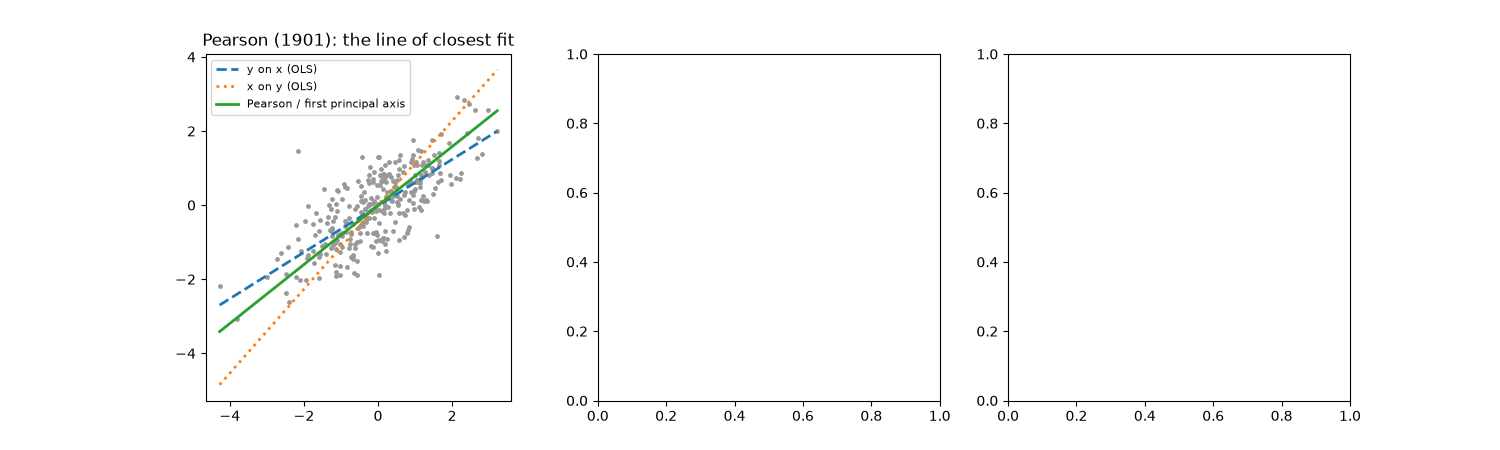
y on x (OLS)                     slope 0.627, perpendicular sum of squares   97.96
x on y (OLS)                     slope 1.135, perpendicular sum of squares  108.00
Pearson / first principal axis   slope 0.796, perpendicular sum of squares   91.04
smallest eigenvalue x (n - 1) =   91.04

<matplotlib.legend.Legend object at 0x112bf5be0>

Hotelling’s components of six test scores

Six scores driven by two hidden abilities, “verbal” and “quantitative”, plus noise. Standardizing (the correlation matrix) puts the tests on an equal footing. Two components carry most of the variance, and their loadings separate the two kinds of test.

n = 500
verbal, quantitative = rng.normal(size=(2, n))
loadings = np.array([[0.9, 0.1], [0.8, 0.2], [0.85, 0.0], [0.1, 0.9], [0.2, 0.8], [0.0, 0.85]])
scores = np.column_stack([verbal, quantitative]) @ loadings.T + 0.4 * rng.normal(size=(n, 6))
tests = ["reading", "vocabulary", "grammar", "arithmetic", "algebra", "geometry"]
hotelling = principal_component_analysis(scores, standardize=True)
print("explained variance ratio:", hotelling.explained_variance_ratio.round(3))

ax1.bar(np.arange(1, 7), hotelling.explained_variance_ratio, color="tab:blue")
ax1.plot(np.arange(1, 7), np.cumsum(hotelling.explained_variance_ratio), "ko-", label="cumulative")
ax1.set_xlabel("component")
ax1.set_ylabel("fraction of variance")
ax1.set_title("Scree plot: two components dominate")
ax1.legend()

first, second = hotelling.components[0], hotelling.components[1]
ax2.axhline(0, color="0.8")
ax2.axvline(0, color="0.8")
for name, a, c in zip(tests, first, second, strict=True):
    ax2.arrow(0, 0, a, c, head_width=0.02, color="tab:red" if name in tests[:3] else "tab:green", length_includes_head=True)
    ax2.annotate(name, (a, c), textcoords="offset points", xytext=(4, 2), fontsize=8)
ax2.set_xlabel("loading on component 1 (general ability)")
ax2.set_ylabel("loading on component 2 (verbal vs. quantitative)")
ax2.set_title("Hotelling (1933): component loadings")
ax2.set_aspect("equal")
fig.tight_layout()

plt.show()

explained variance ratio: [0.539 0.348 0.032 0.031 0.028 0.023]