OLS regression with residual diagnostics

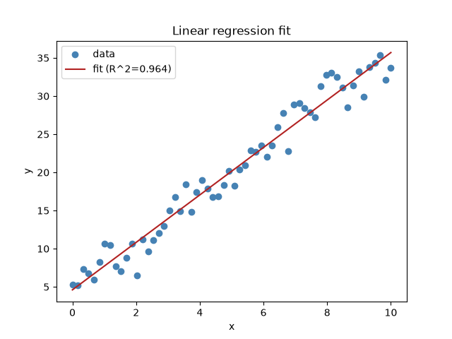
Fits a noisy linear relationship and inspects the fit: coefficient standard errors/p-values, R^2, and a residuals-vs-fitted-values plot.

import numpy as np

from mathematicskit.statistics import linear_regression
from mathematicskit.statistics.visualizers.plots import plot_regression_fit, plot_residuals

Simulate noisy linear data and fit

rng = np.random.default_rng(0)
x = np.linspace(0.0, 10.0, 60)
y = 3.0 * x + 5.0 + rng.normal(0.0, 2.0, x.shape)

result = linear_regression(x, y)
print(f"intercept = {result.coefficients[0]:.3f} (se={result.standard_errors[0]:.3f}, p={result.p_values[0]:.4f})")
print(f"slope     = {result.coefficients[1]:.3f} (se={result.standard_errors[1]:.3f}, p={result.p_values[1]:.4f})")
print(f"R^2 = {result.r_squared:.4f}, adjusted R^2 = {result.adjusted_r_squared:.4f}")

intercept = 4.608 (se=0.458, p=0.0000)
slope     = 3.109 (se=0.079, p=0.0000)
R^2 = 0.9639, adjusted R^2 = 0.9633

Plot the fit and residual diagnostics

plot_regression_fit(x, y, result)
plot_residuals(result)

• 
• 

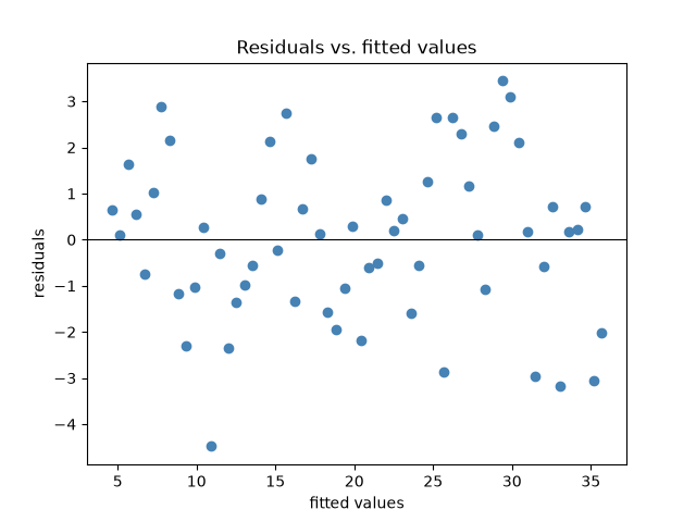
<Axes: title={'center': 'Residuals vs. fitted values'}, xlabel='fitted values', ylabel='residuals'>