Yule’s autoregressive model of the sunspot cycle

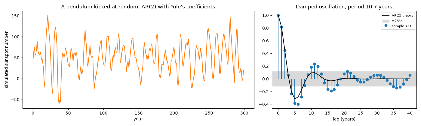
Yule (1927) argued that Wolfer’s sunspot numbers were not a clean sine wave hidden in noise, but a pendulum kicked at random. He fitted

\[X_t = \phi_1 X_{t-1} + \phi_2 X_{t-2} + \varepsilon_t, \qquad \phi_1 \approx 1.34,\ \phi_2 \approx -0.65,\]

the first autoregressive model, and found its period from the roots of \(z^2 - \phi_1 z - \phi_2\). Here a series is simulated from Yule’s coefficients (no sunspot data ship with mathematicskit), and the Yule-Walker equations recover them from the series alone.

import matplotlib.pyplot as plt
import numpy as np

from mathematicskit.statistics import ar_autocorrelation, autocorrelation, simulate_ar, yule_walker

phi = np.array([1.34, -0.65])
years = 300
series = 50 + simulate_ar(phi, n=years, sigma=15.0, seed=1927)

The implied cycle

The characteristic roots are complex, \(r e^{\pm i\theta}\): the model is a damped oscillation with period \(2\pi/\theta\).

roots = np.roots([1.0, -phi[0], -phi[1]])
period = 2 * np.pi / abs(np.angle(roots[0]))
print(f"roots {roots.round(3)}, modulus {abs(roots[0]):.3f}, period {period:.1f} years (sunspot cycle: about 11)")

roots [0.67+0.448j 0.67-0.448j], modulus 0.806, period 10.7 years (sunspot cycle: about 11)

The Yule-Walker fit

fit = yule_walker(series, 2)
fit_period = 2 * np.pi / abs(np.angle(np.roots([1.0, -fit.coefficients[0], -fit.coefficients[1]])[0]))
print(f"fitted phi = {fit.coefficients.round(3)} (true {phi}), noise sd {np.sqrt(fit.noise_variance):.1f} (true 15.0)")
print(f"fitted period {fit_period:.1f} years")
for order in (1, 2, 3, 4):
    print(f"AR({order}) innovation variance: {yule_walker(series, order).noise_variance:7.1f}")

fitted phi = [ 1.362 -0.666] (true [ 1.34 -0.65]), noise sd 15.6 (true 15.0)
fitted period 10.8 years
AR(1) innovation variance:   440.2
AR(2) innovation variance:   244.8
AR(3) innovation variance:   244.4
AR(4) innovation variance:   244.2

Series and autocorrelation

fig, (ax0, ax1) = plt.subplots(1, 2, figsize=(14, 4.2), gridspec_kw={"width_ratios": [1.6, 1]})
ax0.plot(np.arange(years), series, color="tab:orange")
ax0.set_xlabel("year")
ax0.set_ylabel("simulated sunspot number")
ax0.set_title("A pendulum kicked at random: AR(2) with Yule's coefficients")

lags = np.arange(41)
ax1.stem(lags, autocorrelation(series, 40), basefmt=" ", label="sample ACF")
ax1.plot(lags, ar_autocorrelation(phi, 40), "k-", label="AR(2) theory")
ax1.axhspan(-2 / np.sqrt(years), 2 / np.sqrt(years), color="0.85", label=r"$\pm 2/\sqrt{n}$")
ax1.set_xlabel("lag (years)")
ax1.set_title(f"Damped oscillation, period {period:.1f} years")
ax1.legend(fontsize=8)
fig.tight_layout()

plt.show()