The Poincaré-Hopf index theorem (1885-1927)

Walk around a small circle enclosing a zero of a planar vector field, and the field’s direction turns a whole number of times. That number is the zero’s index: \(+1\) for sources, sinks and centres, \(-1\) for saddles. Poincaré (1885) proved that on a closed surface the indices sum to the Euler characteristic, and Hopf (1927) extended this to all dimensions. For a disc, with the field pointing outward on the boundary, the sum is \(\chi(\text{disc}) = 1\). Below, a field with two sources and a saddle gives \(1 + 1 - 1 = 1\).

import matplotlib.pyplot as plt
import numpy as np

from mathematicskit.topology import vector_field_index


def field(x, y):
    """Two sources at x = ±1/2 and a saddle at 0; it points outward on the unit circle."""
    return (x**3 - 0.25 * x, y)


zeros = {"source at (-1/2, 0)": (-0.5, 0.0), "saddle at (0, 0)": (0.0, 0.0), "source at (1/2, 0)": (0.5, 0.0)}
for name, center in zeros.items():
    print(f"{name}: index {vector_field_index(field, center=center, radius=0.15)}")
print("around the unit circle:", vector_field_index(field, radius=1.0), "= chi(disc)")

source at (-1/2, 0): index 1
saddle at (0, 0): index -1
source at (1/2, 0): index 1
around the unit circle: 1 = chi(disc)

The field, the loops, and the turning arrows

x, y = np.meshgrid(np.linspace(-1.1, 1.1, 23), np.linspace(-1.1, 1.1, 23))
u, v = field(x, y)
norm = np.hypot(u, v) + 1e-12
fig, axes = plt.subplots(1, 2, figsize=(12, 5.5))
ax = axes[0]
ax.quiver(x, y, u / norm, v / norm, np.log(norm), cmap="viridis", scale=30)
t = np.linspace(0, 2 * np.pi, 200)
ax.plot(np.cos(t), np.sin(t), "k", lw=2, label="boundary: index 1")
for (cx, cy), color in zip(zeros.values(), ("tab:red", "tab:blue", "tab:red"), strict=True):
    ax.plot(cx + 0.15 * np.cos(t), cy + 0.15 * np.sin(t), color=color, lw=2)
    ax.annotate(f"{vector_field_index(field, center=(cx, cy), radius=0.15):+d}", (cx, cy + 0.2), ha="center", color=color, fontsize=13)
ax.set_aspect("equal")
ax.legend(loc="lower left")
ax.set_title("two sources and a saddle in the disc")

ax = axes[1]
for (name, (cx, cy)), color in zip(zeros.items(), ("tab:red", "tab:blue", "tab:orange"), strict=True):
    fu, fv = field(cx + 0.15 * np.cos(t), cy + 0.15 * np.sin(t))
    ax.plot(t, np.unwrap(np.arctan2(fv, fu)) / (2 * np.pi), color=color, label=name)
fu, fv = field(np.cos(t), np.sin(t))
ax.plot(t, np.unwrap(np.arctan2(fv, fu)) / (2 * np.pi), "k", lw=2, label="unit circle")
ax.set_xlabel("angle around the loop")
ax.set_ylabel("direction of the field / $2\\pi$")
ax.legend()
ax.set_title("each index is the field's net number of turns")
fig.suptitle("Poincaré-Hopf: indices sum to the Euler characteristic")

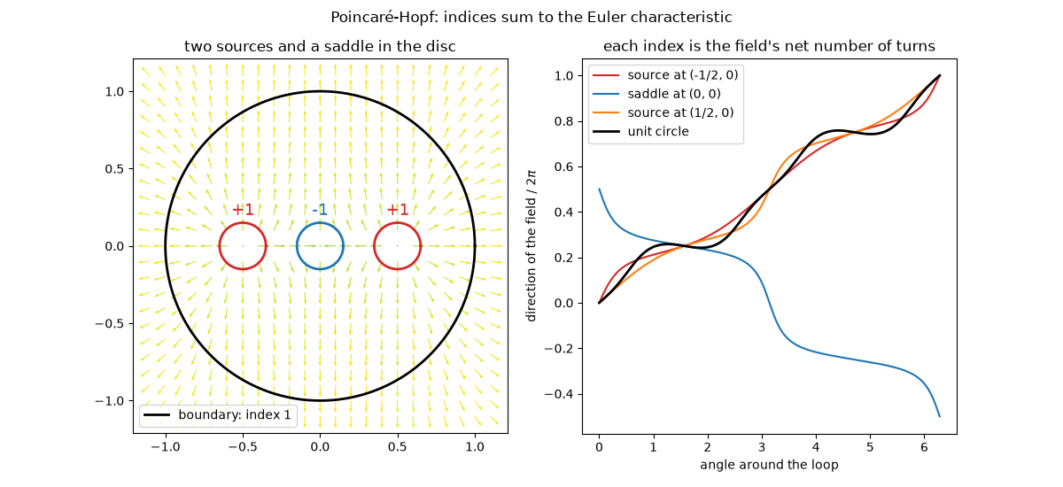
Text(0.5, 0.98, 'Poincaré-Hopf: indices sum to the Euler characteristic')