Litterman-Scheinkman: level, slope, curvature

Litterman and Scheinkman (1991) ran a principal component analysis of Treasury returns and found that three factors explain almost all of the variation. They named them level, steepness (slope) and curvature. The script repeats the analysis on synthetic daily yield changes and shows the three loadings and their shares of variance.

import matplotlib.pyplot as plt
import numpy as np

from financialkit.fixed_income import simulate_yield_changes, yield_curve_pca
from financialkit.fixed_income.visualizers import plot_pca_loadings

tenors = np.array([0.25, 0.5, 1, 2, 3, 5, 7, 10, 20, 30])
changes = simulate_yield_changes(tenors, n_obs=2500, rng=1991)
pca = yield_curve_pca(changes, tenors)

Loadings of the first three components

plot_pca_loadings(pca)

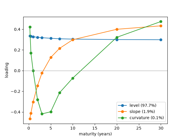
<Axes: xlabel='maturity (years)', ylabel='loading'>

Share of variance explained

fig, ax = plt.subplots()
ax.bar(np.arange(1, tenors.size + 1), 100 * pca.explained_variance_ratio)
ax.plot(np.arange(1, tenors.size + 1), 100 * np.cumsum(pca.explained_variance_ratio), "ko-", label="cumulative")
ax.set_xlabel("component")
ax.set_ylabel("variance explained (%)")
ax.legend()
print("first three components explain", f"{100 * pca.explained_variance_ratio[:3].sum():.1f}%")
plt.show()

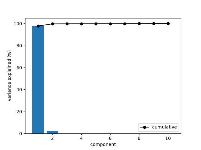
first three components explain 99.7%