Nelson-Siegel

Nelson and Siegel (1987) described the whole yield curve with four numbers:

\[r(t) = \beta_0 + \beta_1 \frac{1-e^{-t/\tau}}{t/\tau} + \beta_2\left(\frac{1-e^{-t/\tau}}{t/\tau} - e^{-t/\tau}\right).\]

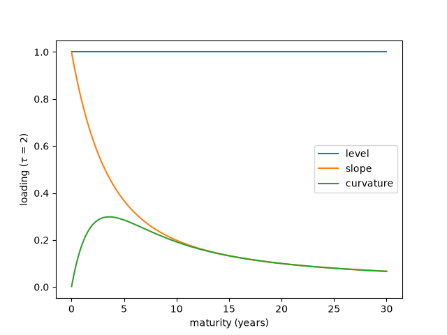
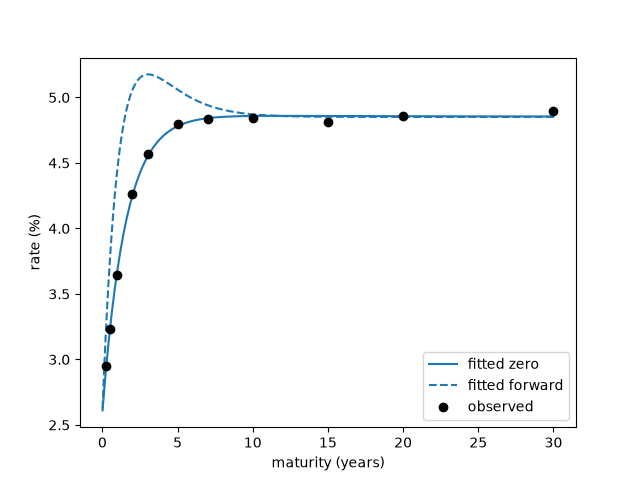
The three loadings are a level, a slope that decays from 1 to 0, and a hump. The script plots them and fits the model to noisy yields.

import matplotlib.pyplot as plt
import numpy as np

from financialkit.fixed_income import NelsonSiegelCurve, fit_nelson_siegel
from financialkit.fixed_income.visualizers import plot_yield_curve

The three loadings

t = np.linspace(0.01, 30, 300)
fig, ax = plt.subplots()
for name, curve in (("level", NelsonSiegelCurve(1, 0, 0, 2.0)), ("slope", NelsonSiegelCurve(0, 1, 0, 2.0)), ("curvature", NelsonSiegelCurve(0, 0, 1, 2.0))):
    ax.plot(t, curve.zero_rate(t), label=name)
ax.set_xlabel("maturity (years)")
ax.set_ylabel(r"loading ($\tau$ = 2)")
ax.legend()

<matplotlib.legend.Legend object at 0x116f0d6a0>

Fit to noisy yields

rng = np.random.default_rng(1987)
tenors = np.array([0.25, 0.5, 1, 2, 3, 5, 7, 10, 15, 20, 30])
true = NelsonSiegelCurve(0.048, -0.022, 0.025, 1.6)
observed = true.zero_rate(tenors) + rng.normal(0, 0.0005, tenors.size)
fit = fit_nelson_siegel(tenors, observed)
print("fitted [b0, b1, b2, tau]:", fit.params.round(4), f"RMSE {1e4 * fit.rmse:.1f} bp")
ax = plot_yield_curve(fit.curve, label="fitted")
ax.plot(tenors, 100 * observed, "ko", label="observed")
ax.legend()
plt.show()

fitted [b0, b1, b2, tau]: [ 0.0485 -0.0225  0.0233  1.5472] RMSE 2.4 bp