Carleton-Cooper bootstrapping

With bonds that pay on common dates, Carleton and Cooper (1976) noted that prices are linear in the discount factors, \(P = C d\). Solving that system one bond at a time, shortest first, is bootstrapping: each bond adds one zero rate at its maturity. With more bonds than dates the same system is solved by least squares.

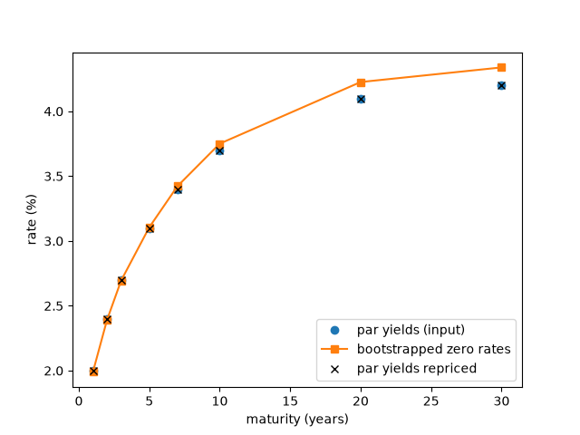
The first cell reproduces Hull’s bootstrapping table. The second strips a zero curve from par rates. The third recovers discount factors from a noisy, overdetermined set of prices.

import matplotlib.pyplot as plt
import numpy as np

from financialkit.fixed_income import bootstrap_par_curve, bootstrap_zero_curve, carleton_cooper_discount_factors

Hull’s Tables 4.3-4.4

T = [0.25, 0.5, 1.0, 1.5, 2.0]
curve = bootstrap_zero_curve(T, [0, 0, 0, 0.08, 0.12], [97.5, 94.9, 90.0, 96.0, 101.6])
for t, r in zip(curve.tenors, curve.rates, strict=True):
    print(f"{t:4.2f} years: {100 * r:.3f}%")

0.25 years: 10.127%
0.50 years: 10.469%
1.00 years: 10.536%
1.50 years: 10.681%
2.00 years: 10.808%

A zero curve from par yields

tenors = np.array([1, 2, 3, 5, 7, 10, 20, 30.0])
par = np.array([0.020, 0.024, 0.027, 0.031, 0.034, 0.037, 0.041, 0.042])
zc = bootstrap_par_curve(tenors, par)
fig, ax = plt.subplots()
ax.plot(tenors, 100 * par, "o", label="par yields (input)")
ax.plot(zc.tenors, 100 * zc.rates, "s-", label="bootstrapped zero rates")
ax.plot(tenors, 100 * zc.par_yield(tenors), "x", color="k", label="par yields repriced")
ax.set_xlabel("maturity (years)")
ax.set_ylabel("rate (%)")
ax.legend()

<matplotlib.legend.Legend object at 0x116f0d400>

Least squares with more bonds than dates

rng = np.random.default_rng(1976)
dates = np.arange(1, 6, dtype=float)
d_true = np.exp(-0.035 * dates)
C = np.zeros((30, dates.size))
for i in range(30):
    n = rng.integers(1, dates.size + 1)
    C[i, :n] = 100 * rng.uniform(0.01, 0.08)
    C[i, n - 1] += 100.0
prices = C @ d_true + rng.normal(0, 0.02, 30)
res = carleton_cooper_discount_factors(dates, C, prices)
print("estimated:", res.params.round(5))
print("true:     ", d_true.round(5))
plt.show()

estimated: [0.96569 0.93238 0.90028 0.86937 0.83943]
true:      [0.96561 0.93239 0.90032 0.86936 0.83946]