McCulloch’s spline discount function

Huston McCulloch (1971) fitted the discount function itself with a spline, \(d(t) = 1 + \sum_j a_j g_j(t)\). Because every bond price is linear in \(d\), it is also linear in the coefficients, so the fit is ordinary least squares on a cross-section of bond prices. His 1971 paper used quadratic splines; the cubic version (1975) gives smooth forward rates.

import matplotlib.pyplot as plt
import numpy as np

from financialkit.fixed_income import NelsonSiegelCurve, bond_cash_flows, fit_mcculloch_spline

rng = np.random.default_rng(1971)
true = NelsonSiegelCurve(0.05, -0.03, 0.02, 1.5)

A noisy cross-section of 40 coupon bonds

maturities = np.sort(rng.uniform(0.3, 25, 40))
coupons = np.round(rng.uniform(0.01, 0.07, 40), 3)
bonds = [bond_cash_flows(100.0, c, T) for c, T in zip(coupons, maturities, strict=True)]
prices = np.array([b.present_value(true) for b in bonds]) + rng.normal(0, 0.05, 40)

Quadratic and cubic fits

knots = [1.0, 3.0, 7.0, 15.0]
t = np.linspace(0.1, 25, 300)
fig, axes = plt.subplots(1, 2, figsize=(10, 4))
axes[0].plot(t, true.discount(t), "k", lw=3, alpha=0.3, label="true")
axes[1].plot(t, 100 * true.zero_rate(t), "k", lw=3, alpha=0.3, label="true")
for degree in (2, 3):
    res = fit_mcculloch_spline(bonds, prices, knots=knots, degree=degree)
    print(f"degree {degree}: price RMSE {res.rmse:.4f}")
    axes[0].plot(t, res.curve.discount(t), label=f"degree {degree}")
    axes[1].plot(t, 100 * res.curve.zero_rate(t), label=f"degree {degree}")
for k in knots:
    axes[0].axvline(k, color="0.85", lw=0.8)
axes[0].set_ylabel("discount factor d(t)")
axes[1].set_ylabel("zero rate (%)")
for ax in axes:
    ax.set_xlabel("maturity (years)")
    ax.legend()
plt.show()

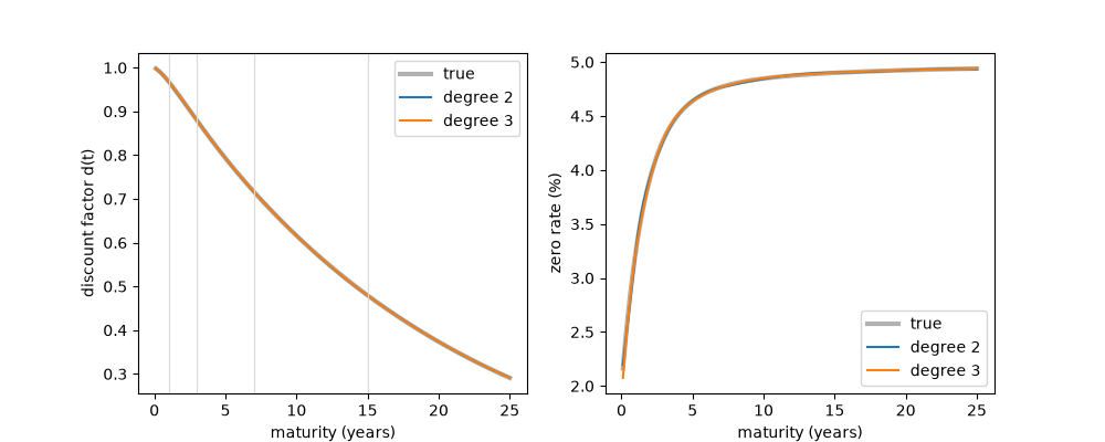
degree 2: price RMSE 0.0513
degree 3: price RMSE 0.0434