Hicks: duration as an elasticity (modified duration)

John Hicks (1939) found Macaulay’s average period again as the elasticity of a capital value with respect to the discount factor. Measured per unit of yield, that elasticity is modified duration,

\[D_{mod} = -\frac{1}{P}\frac{dP}{dy} = \frac{D_{mac}}{1 + y/m},\]

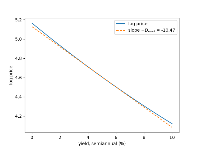
for a yield compounded \(m\) times a year. The script checks the relation across compounding frequencies and shows that \(-D_{mod}\) is the slope of the log-price curve.

import matplotlib.pyplot as plt
import numpy as np

from financialkit.fixed_income import bond_cash_flows, macaulay_duration, modified_duration, price_from_yield

cf = bond_cash_flows(100.0, 0.05, 15.0, freq=2)
y0 = 0.05

Macaulay and modified duration by compounding frequency

for m in (1, 2, 4, 12, None):
    d_mac = macaulay_duration(cf, y0, m)
    d_mod = modified_duration(cf, y0, m)
    ratio = 1.0 if m is None else 1 + y0 / m
    print(f"m={str(m):>4}: D_mac={d_mac:.4f}  D_mod={d_mod:.4f}  D_mac/(1+y/m)={d_mac / ratio:.4f}")

m=   1: D_mac=10.7423  D_mod=10.2308  D_mac/(1+y/m)=10.2308
m=   2: D_mac=10.7268  D_mod=10.4651  D_mac/(1+y/m)=10.4651
m=   4: D_mac=10.7188  D_mod=10.5865  D_mac/(1+y/m)=10.5865
m=  12: D_mac=10.7134  D_mod=10.6689  D_mac/(1+y/m)=10.6689
m=None: D_mac=10.7107  D_mod=10.7107  D_mac/(1+y/m)=10.7107

Modified duration is the slope of log-price against yield

y = np.linspace(0.0, 0.10, 200)
log_p = np.log(price_from_yield(cf, y, 2))
d_mod = modified_duration(cf, y0, 2)
p0 = np.log(price_from_yield(cf, y0, 2))
fig, ax = plt.subplots()
ax.plot(100 * y, log_p, label="log price")
ax.plot(100 * y, p0 - d_mod * (y - y0), ls="--", label=f"slope $-D_{{mod}}$ = {-d_mod:.2f}")
ax.set_xlabel("yield, semiannual (%)")
ax.set_ylabel("log price")
ax.legend()
plt.show()