Ho’s key rate durations

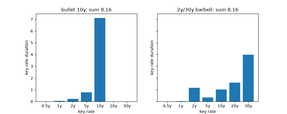
A single duration assumes the whole curve moves in parallel. Thomas Ho (1992) shocked the curve one key rate at a time, with triangular shapes that sum to a parallel shift, so a bond’s risk becomes a vector whose entries add up to its effective duration. Two portfolios with the same duration can have very different key rate profiles.

import matplotlib.pyplot as plt
import numpy as np

from financialkit.fixed_income import NelsonSiegelCurve, bond_cash_flows, key_rate_durations, key_rate_weights, redington_immunize
from financialkit.fixed_income.visualizers import plot_key_rate_durations

keys = np.array([0.5, 1, 2, 5, 10, 20, 30])
curve = NelsonSiegelCurve(0.045, -0.02, 0.01, 2.0)

The key-rate shock shapes

t = np.linspace(0, 35, 400)
fig, ax = plt.subplots()
for k, w in zip(keys, key_rate_weights(t, keys), strict=True):
    ax.plot(t, w, label=f"{k:g}y")
ax.set_xlabel("maturity (years)")
ax.set_ylabel("shock weight")
ax.legend(ncol=4)

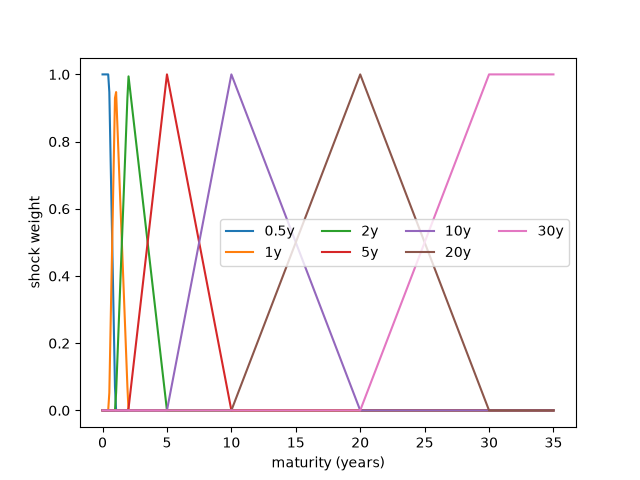
<matplotlib.legend.Legend object at 0x117062ba0>

Bullet and barbell with equal duration

bullet = bond_cash_flows(100.0, 0.045, 10.0)
target = bullet.scaled(1.0)
barbell = redington_immunize(target, [bond_cash_flows(1.0, 0.04, 2.0), bond_cash_flows(1.0, 0.05, 30.0)], curve).portfolio
fig, axes = plt.subplots(1, 2, figsize=(10, 4), sharey=True)
for ax, (name, cf) in zip(axes, (("bullet 10y", bullet), ("2y/30y barbell", barbell)), strict=True):
    res = key_rate_durations(cf, curve, keys)
    plot_key_rate_durations(res, ax=ax)
    ax.set_title(f"{name}: sum {res.durations.sum():.2f}")
plt.show()