Ho-Lee: the first arbitrage-free term-structure model

Thomas Ho and Sang-Bin Lee (1986) turned the problem around. Instead of deriving a curve from a short-rate model, they took today’s curve as given and made the model fit it: a binomial tree of whole discount curves whose drift is chosen to reprice every bond. Its continuous-time limit is Merton’s Gaussian rate with a time-dependent drift,

\[dr = \theta(t)\,dt + \sigma\,dW, \qquad \theta(t) = \partial_t f(0, t) + \sigma^2 t,\]

so any initial curve is matched exactly and every interest-rate derivative is priced relative to it.

import matplotlib.pyplot as plt
import numpy as np

from financialkit.fixed_income import NelsonSiegelCurve
from financialkit.fixed_income.visualizers import plot_yield_curve
from financialkit.interest_rate_models import HoLeeModel, VasicekModel, monte_carlo_bond_prices

curve = NelsonSiegelCurve(0.05, -0.025, 0.02, 1.5)  # a humped market curve
model = HoLeeModel(curve, sigma=0.01)

An equilibrium model cannot fit the market

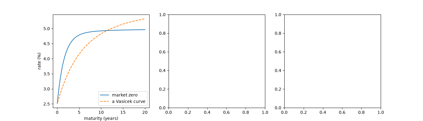
The best a Vasicek curve can do is a smooth monotone or single-hump shape tied to its own parameters; Ho-Lee reproduces the market curve by construction.

fig, axes = plt.subplots(1, 3, figsize=(14, 4))
plot_yield_curve(curve, t_max=20, ax=axes[0], label="market", show_forward=False)
T = np.linspace(0.1, 20, 200)
axes[0].plot(T, 100 * VasicekModel(0.025, 0.3, 0.06, 0.015).yields(T), "--", label="a Vasicek curve")
axes[0].legend()

<matplotlib.legend.Legend object at 0x11a3d8ad0>

The drift that fits the curve

t = np.linspace(0.0, 20, 200)
axes[1].plot(t, 100 * model.theta(t), label=r"$\theta(t)$")
axes[1].plot(t, 100 * curve.instantaneous_forward(t), label="f(0, t)")
axes[1].plot(t, 100 * model.shift(t), label=r"E[r(t)] = f(0,t) + $\sigma^2 t^2/2$")
axes[1].set_xlabel("t (years)")
axes[1].set_ylabel("% per year")
axes[1].legend()

<matplotlib.legend.Legend object at 0x11a3d9010>

Simulated rates reprice every market bond

res = monte_carlo_bond_prices(model, np.arange(1.0, 21.0), n_steps=200, n_paths=8000, rng=0)
axes[2].plot(res.maturities, 100 * curve.zero_rate(res.maturities), "k-", label="market zero curve")
axes[2].plot(res.maturities, 100 * -np.log(res.prices) / res.maturities, "o", ms=3, label="Ho-Lee Monte Carlo")
axes[2].set_xlabel("maturity (years)")
axes[2].set_ylabel("zero yield (%)")
axes[2].legend()
print(f"largest |z| across 20 maturities: {np.abs(res.z_scores).max():.2f}")
fig.tight_layout()

plt.show()

largest |z| across 20 maturities: 1.50