Hull-White: extended Vasicek

John Hull and Alan White (1990) combined Vasicek’s mean reversion with Ho and Lee’s curve fitting,

\[dr = (\theta(t) - a r)\,dt + \sigma\,dW.\]

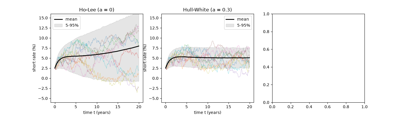
The initial curve is matched exactly, and mean reversion makes the volatility of a \(\tau\)-year yield decay like \(B(\tau)/\tau = (1 - e^{-a\tau})/(a\tau)\), as observed, instead of staying flat as in Ho-Lee. The model became the industry’s workhorse for Bermudan swaptions and callable bonds.

import matplotlib.pyplot as plt
import numpy as np

from financialkit.fixed_income import NelsonSiegelCurve
from financialkit.interest_rate_models import HoLeeModel, HullWhiteModel, monte_carlo_bond_prices
from financialkit.interest_rate_models.visualizers import plot_short_rate_paths

curve = NelsonSiegelCurve(0.05, -0.025, 0.02, 1.5)

Mean reversion tames the rate’s spread

fig, axes = plt.subplots(1, 3, figsize=(14, 4))
for a, ax in ((0.0, axes[0]), (0.3, axes[1])):
    model = HullWhiteModel(curve, a, 0.012) if a else HoLeeModel(curve, 0.012)
    times, r = model.simulate(20.0, 200, 3000, rng=0)
    plot_short_rate_paths(times, r, n_show=10, ax=ax)
    ax.set_ylim(-6, 16)
    ax.set_title("Ho-Lee (a = 0)" if a == 0 else f"Hull-White (a = {a})")

The term structure of yield volatility

tau = np.linspace(0.1, 30, 200)
for a in (0.0, 0.05, 0.2, 0.5):
    vol = np.ones_like(tau) if a == 0 else -np.expm1(-a * tau) / (a * tau)
    axes[2].plot(tau, 100 * 0.012 * vol, label=f"a = {a}")
axes[2].set_xlabel("yield maturity (years)")
axes[2].set_ylabel("instantaneous yield volatility (%)")
axes[2].legend()
fig.tight_layout()

Fitted to the curve, and Vasicek’s bond formula at later dates

hw = HullWhiteModel(curve, 0.3, 0.012)
res = monte_carlo_bond_prices(hw, [1.0, 5.0, 10.0, 20.0], n_steps=200, n_paths=8000, rng=1)
for T, z in zip(res.maturities, res.z_scores, strict=True):
    print(f"T = {T:4.0f}: market P = {curve.discount(T):.5f}, Monte Carlo z = {z:+.2f}")
print("P(5, 10) at r(5) = 3%, 5%, 7%:", np.round(hw.zero_coupon_bond(10.0, t=5.0, state=np.array([0.03, 0.05, 0.07])), 5))

plt.show()

T =    1: market P = 0.96456, Monte Carlo z = -0.11
T =    5: market P = 0.78726, Monte Carlo z = -0.19
T =   10: market P = 0.61125, Monte Carlo z = -0.18
T =   20: market P = 0.37065, Monte Carlo z = -0.58
P(5, 10) at r(5) = 3%, 5%, 7%: [0.82022 0.77882 0.73951]