Black-Derman-Toy: a lognormal rate tree

Fischer Black, Emanuel Derman and William Toy (1990), at Goldman Sachs, built a binomial tree of short rates that is lognormal, so rates stay positive, and fitted to the market curve level by level. At step \(i\) the rates are \(r_{i,j} = U_i e^{\sigma_i\sqrt{\Delta t}\,(2j - i)}\) with probability 1/2 on each branch, and the median \(U_i\) is solved so that the tree reprices the bond maturing one step later, using Arrow-Debreu prices carried forward through the tree. Options, including American ones, are then priced by backward induction.

import matplotlib.pyplot as plt
import numpy as np

from financialkit.fixed_income import NelsonSiegelCurve
from financialkit.interest_rate_models import black_derman_toy_tree
from financialkit.interest_rate_models.visualizers import plot_rate_tree

curve = NelsonSiegelCurve(0.05, -0.025, 0.02, 1.5)

A small tree

small = black_derman_toy_tree(curve, 0.2, 5.0, 10)
fig, axes = plt.subplots(1, 3, figsize=(14, 4))
plot_rate_tree(small, ax=axes[0])
axes[0].set_title("BDT tree, 10 steps, 20% rate volatility")

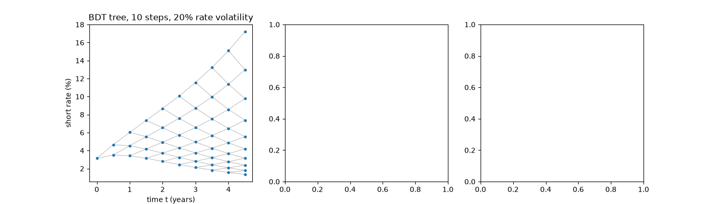
Text(0.5, 1.0, 'BDT tree, 10 steps, 20% rate volatility')

Calibrated to the curve by forward induction

tree = black_derman_toy_tree(curve, 0.2, 10.0, 200)
T = tree.times[1:]
model_P = np.array([tree.zero_coupon_bond(t) for t in T[::10]])
print(f"largest repricing error over 20 bonds: {np.max(np.abs(model_P / curve.discount(T[::10]) - 1)):.1e}")
axes[1].plot(T, 100 * curve.zero_rate(T), "k-", label="market zero curve")
axes[1].plot(T[::10], 100 * -np.log(model_P) / T[::10], "o", ms=4, label="BDT tree")
median = np.array([np.exp(np.mean(np.log(tree.rates[i, : i + 1]))) for i in range(tree.n_steps)])  # the U_i
axes[1].plot(tree.times[:-1], 100 * median, ":", label="median short rate")
axes[1].set_xlabel("maturity (years)")
axes[1].set_ylabel("%")
axes[1].legend()

largest repricing error over 20 bonds: 4.4e-16

<matplotlib.legend.Legend object at 0x11a79ee40>

European and American options on a bond

Puts expiring in 3 years on a bond maturing in 10. The American put is exercised early when rates jump, so it is worth more.

K = np.linspace(0.6, 0.8, 9)
euro = [tree.bond_option(3.0, 10.0, k, "put") for k in K]
amer = [tree.bond_option(3.0, 10.0, k, "put", american=True) for k in K]
axes[2].plot(K, euro, "o-", label="European put")
axes[2].plot(K, amer, "s-", label="American put")
axes[2].set_xlabel("strike (per unit face)")
axes[2].set_ylabel("option value")
axes[2].legend()
fig.tight_layout()

plt.show()