Duffie-Kan: affine term structures

Darrell Duffie and Rui Kan (1996) found the common structure behind Vasicek, CIR and their multi-factor extensions. If the state’s drift and variance are affine in the state,

\[dX = (K_0 + K_1 X)\,dt + \operatorname{diag}(\sigma)\sqrt{\alpha + \beta X}\,dW, \qquad r = \delta_0 + \delta_1 \cdot X,\]

then bonds are exponential-affine, \(P = e^{A(\tau) + B(\tau)\cdot X}\), with \(A\) and \(B\) the solutions of Riccati ODEs. One solver prices the whole family; here scipy.integrate.solve_ivp() recovers the Vasicek and CIR closed forms and then prices a two-factor model with no closed form at all.

import matplotlib.pyplot as plt
import numpy as np

from financialkit.interest_rate_models import AffineModel, CIRModel, VasicekModel, monte_carlo_bond_prices

T = np.linspace(0.25, 30, 120)

The Riccati ODEs recover Vasicek and CIR

fig, axes = plt.subplots(1, 3, figsize=(14, 4))
for name, affine, closed in (
    ("Vasicek", AffineModel.vasicek(0.02, 0.3, 0.05, 0.015), VasicekModel(0.02, 0.3, 0.05, 0.015)),
    ("CIR", AffineModel.cir(0.02, 0.3, 0.05, 0.1), CIRModel(0.02, 0.3, 0.05, 0.1)),
):
    err = np.abs(affine.zero_coupon_bond(T) / closed.zero_coupon_bond(T) - 1)
    axes[0].semilogy(T, np.maximum(err, 1e-16), label=name)
    print(f"{name}: largest relative error {err.max():.1e}")
axes[0].set_xlabel("maturity (years)")
axes[0].set_ylabel("|Riccati / closed form - 1|")
axes[0].legend()

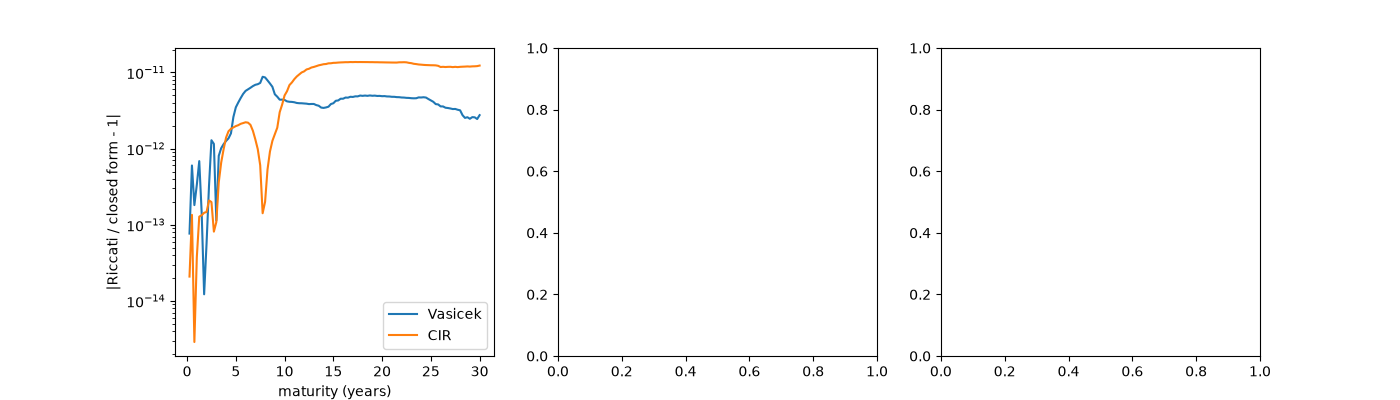
Vasicek: largest relative error 8.8e-12
CIR: largest relative error 1.4e-11

<matplotlib.legend.Legend object at 0x11a79f380>

A two-factor model: a Gaussian factor plus a square-root factor

The Gaussian factor reverts fast and feeds the square-root factor’s drift through \(K_1\), which no product of one-factor formulas can capture.

model = AffineModel(
    x0=[-0.01, 0.03],
    K0=[0.0, 0.3 * 0.04],
    K1=[[-1.0, 0.0], [0.2, -0.3]],
    sigma=[0.012, 0.08],
    alpha=[1.0, 0.0],
    beta=[[0.0, 0.0], [0.0, 1.0]],
    delta0=0.0,
    delta1=[1.0, 1.0],
)
A, B = model.riccati(T)
axes[1].plot(T, -B[:, 0] / T, label="Gaussian factor")
axes[1].plot(T, -B[:, 1] / T, label="square-root factor")
axes[1].set_xlabel("maturity (years)")
axes[1].set_ylabel(r"yield loading $-B_k(\tau)/\tau$")
axes[1].legend()

for x0 in ([-0.01, 0.03], [0.01, 0.03], [0.0, 0.06]):
    axes[2].plot(T, 100 * -np.log(model.zero_coupon_bond(T, t=0.0, state=x0)) / T, label=f"x = {x0}")
axes[2].set_xlabel("maturity (years)")
axes[2].set_ylabel("zero yield (%)")
axes[2].legend()
fig.tight_layout()

Riccati prices against simulation

res = monte_carlo_bond_prices(model, [1.0, 3.0, 5.0], n_steps=100, n_paths=8000, rng=0)
for t, p, se, ex in zip(res.maturities, res.prices, res.std_errors, res.exact, strict=True):
    print(f"T = {t:.0f}: Riccati {ex:.5f}, Monte Carlo {p:.5f} +/- {se:.5f}")

plt.show()

T = 1: Riccati 0.97596, Monte Carlo 0.97583 +/- 0.00010
T = 3: Riccati 0.91656, Monte Carlo 0.91620 +/- 0.00037
T = 5: Riccati 0.85421, Monte Carlo 0.85379 +/- 0.00060