Brigo-Mercurio G2++: two Gaussian factors

In a one-factor model a single shock moves every yield, so the 1-year and 30-year rates are perfectly correlated, which the data flatly reject. Damiano Brigo and Fabio Mercurio’s G2++ (2001) adds a second Gaussian factor,

\[r = x + y + \varphi(t), \quad dx = -a x\,dt + \sigma\,dW_1, \quad dy = -b y\,dt + \eta\,dW_2, \quad dW_1 dW_2 = \rho\,dt,\]

with \(\varphi\) fitted to today’s curve. Bonds and bond options stay in closed form, and a negative \(\rho\) between a fast and a slow factor decorrelates the ends of the curve.

import matplotlib.pyplot as plt
import numpy as np

from financialkit.fixed_income import NelsonSiegelCurve
from financialkit.interest_rate_models import G2PlusPlusModel, monte_carlo_bond_prices

curve = NelsonSiegelCurve(0.045, -0.02, 0.01, 2.0)
model = G2PlusPlusModel(curve, a=0.8, sigma=0.012, b=0.05, eta=0.008, rho=-0.75)

Correlation between yields

taus = np.array([0.5, 1, 2, 5, 10, 20, 30])
fig, axes = plt.subplots(1, 3, figsize=(14, 4))
im = axes[0].imshow(model.yield_correlation(taus[:, None], taus[None, :]), vmin=0, vmax=1, cmap="viridis")
axes[0].set_xticks(range(taus.size), [f"{t:g}" for t in taus])
axes[0].set_yticks(range(taus.size), [f"{t:g}" for t in taus])
axes[0].set_title("instantaneous yield correlation")
fig.colorbar(im, ax=axes[0])
print(f"corr(1y, 30y): G2++ {model.yield_correlation(1.0, 30.0):.2f}; any one-factor model 1.00")

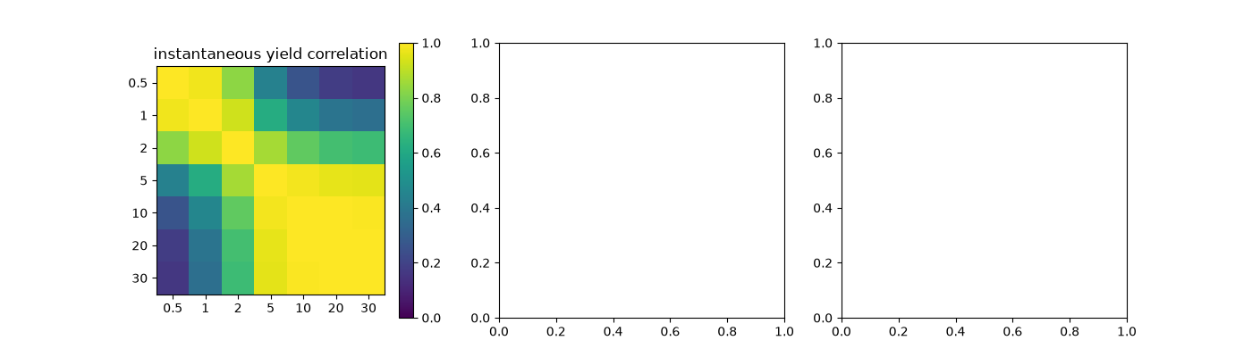
corr(1y, 30y): G2++ 0.37; any one-factor model 1.00

The same correlation from simulated yield changes

_, xy = model.simulate_factors(1.0, 50, 4000, rng=0)
dx = xy[:, 1, :] - xy[:, 0, :]  # factor moves over the first step


def dyield(tau):
    """Change in the tau-year yield, -d ln P / tau = (B_a dx + B_b dy) / tau."""
    Ba, Bb = -np.expm1(-model.a * tau) / model.a, -np.expm1(-model.b * tau) / model.b
    return (Ba * dx[:, 0] + Bb * dx[:, 1]) / tau


axes[1].scatter(1e4 * dyield(1.0), 1e4 * dyield(30.0), s=2, alpha=0.3)
axes[1].set_xlabel("1y yield change (bp)")
axes[1].set_ylabel("30y yield change (bp)")
axes[1].set_title(f"sample corr {np.corrcoef(dyield(1.0), dyield(30.0))[0, 1]:.2f}")

Text(0.5, 1.0, 'sample corr 0.37')

The fitted model reprices the curve

res = monte_carlo_bond_prices(model, np.arange(1.0, 11.0), n_steps=100, n_paths=8000, rng=1)
axes[2].plot(res.maturities, 100 * -np.log(res.exact) / res.maturities, "k-", label="initial curve")
yield_se = 100 * res.std_errors / res.prices / res.maturities
axes[2].errorbar(res.maturities, 100 * -np.log(res.prices) / res.maturities, yerr=1.96 * yield_se, fmt="o", ms=3, label="G2++ Monte Carlo")
axes[2].set_xlabel("maturity (years)")
axes[2].set_ylabel("zero yield (%)")
axes[2].legend()
fig.tight_layout()

plt.show()