Metropolis-Ulam: the Monte Carlo method

Stanislaw Ulam, convalescing in 1946 and playing solitaire, wondered whether it was quicker to estimate his chance of winning by playing many games than by combinatorics. With John von Neumann and Nicholas Metropolis he turned the idea into a method for the neutron-diffusion problems at Los Alamos, and Metropolis and Ulam named it in 1949. An integral is an expectation, so

\[\int_{[0,1)^d} f(u)\,du \approx \frac1n \sum_{i=1}^n f(U_i), \qquad \mathrm{SE} = \frac{s}{\sqrt n},\]

whatever the dimension \(d\).

import matplotlib.pyplot as plt
import numpy as np

from financialkit.monte_carlo import monte_carlo_integrate
from financialkit.monte_carlo.visualizers import plot_confidence_intervals, plot_error_convergence

Throwing darts at the unit square

A point lands inside the quarter disc with probability \(\pi / 4\).

rng = np.random.default_rng(0)
u = rng.random((2000, 2))
inside = np.sum(u**2, axis=1) < 1
res = monte_carlo_integrate(lambda x: 4.0 * (np.sum(x**2, axis=1) < 1), 2000, dim=2, rng=0)
print(f"pi ~ {res.estimate:.4f} +/- {res.std_error:.4f}, 95% CI ({res.ci[0]:.4f}, {res.ci[1]:.4f})")

fig, axes = plt.subplots(1, 3, figsize=(14, 4))
axes[0].scatter(*u[inside].T, s=2, color="C0")
axes[0].scatter(*u[~inside].T, s=2, color="C3")
axes[0].set_aspect("equal")
axes[0].set_title(f"2000 darts: pi ~ {res.estimate:.3f}")

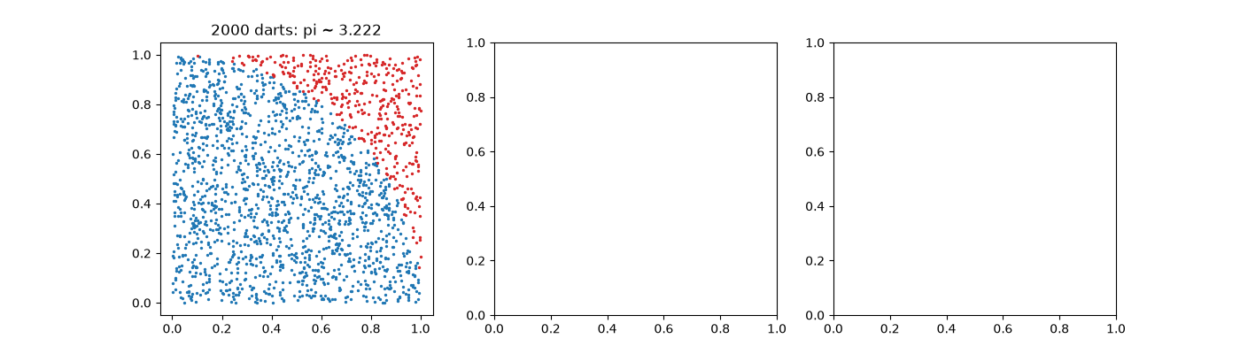
pi ~ 3.2220 +/- 0.0354, 95% CI (3.1526, 3.2914)

Text(0.5, 1.0, '2000 darts: pi ~ 3.222')

The error falls like \(1/\sqrt n\) in any dimension

The volume of the unit ball in 6 dimensions, \(\pi^3/6\), from the cube \([-1, 1]^6\): same rate, larger constant.

ns = np.array([1_000, 4_000, 16_000, 64_000, 256_000])
for d, exact in [(2, np.pi), (6, np.pi**3 / 6)]:
    errs = [abs(monte_carlo_integrate(lambda x: 2.0**d * (np.sum((2 * x - 1) ** 2, axis=1) < 1), n, dim=d, rng=n).estimate - exact) / exact for n in ns]
    plot_error_convergence(ns, errs, ax=axes[1], label=f"ball volume, d = {d}", rates=(0.5,) if d == 2 else ())
axes[1].set_ylabel("relative error")

Text(520.6633986928106, 0.5, 'relative error')

Confidence intervals cover the truth 95% of the time

runs = [monte_carlo_integrate(lambda x: 4.0 * (np.sum(x**2, axis=1) < 1), 1000, dim=2, rng=s) for s in range(60)]
plot_confidence_intervals(runs, exact=np.pi, ax=axes[2])
fig.tight_layout()
plt.show()