Box-Muller normal variates

Every Black-Scholes simulation needs normal random numbers, and a computer produces uniforms. George Box and Mervin Muller (1958) gave an exact transform: if \(u_1, u_2\) are independent uniforms,

\[z_1 = \sqrt{-2\ln u_1}\cos(2\pi u_2), \qquad z_2 = \sqrt{-2\ln u_1}\sin(2\pi u_2)\]

are independent standard normals. The squared radius of a standard bivariate normal is exponential with mean 2 and its angle is uniform, so inverting both gives the pair.

import matplotlib.pyplot as plt
import numpy as np
from scipy.stats import kstest, norm

from financialkit.monte_carlo import box_muller, box_muller_normals

rng = np.random.default_rng(0)
u1, u2 = rng.random((2, 3000))
z1, z2 = box_muller(1.0 - u1, u2)

Uniform square to normal plane

Colouring each uniform pair by its angle \(2\pi u_2\) shows the map: \(u_2\) sets the direction and \(u_1\) the radius.

fig, axes = plt.subplots(1, 3, figsize=(14, 4))
axes[0].scatter(u1, u2, c=u2, s=3, cmap="twilight")
axes[0].set_title("uniforms $(u_1, u_2)$")
axes[1].scatter(z1, z2, c=u2, s=3, cmap="twilight")
axes[1].set_aspect("equal")
axes[1].set_title("Box-Muller $(z_1, z_2)$")

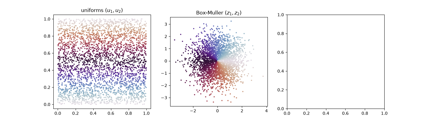
Text(0.5, 1.0, 'Box-Muller $(z_1, z_2)$')

The output is normal

z = box_muller_normals(100_000, rng=1)
x = np.linspace(-4, 4, 200)
axes[2].hist(z, bins=80, density=True, alpha=0.6, label="Box-Muller")
axes[2].plot(x, norm.pdf(x), "k", label="N(0, 1)")
axes[2].legend()
axes[2].set_title(f"KS p-value {kstest(z, 'norm').pvalue:.2f}")
print(f"mean {z.mean():+.4f}, variance {z.var():.4f}, corr(z1, z2) {np.corrcoef(z1, z2)[0, 1]:+.4f}")
fig.tight_layout()
plt.show()

mean +0.0029, variance 0.9990, corr(z1, z2) +0.0012