Boyle: options by Monte Carlo

Phelim Boyle (1977) observed that risk-neutral valuation turns an option price into an expectation, and so into a simulation:

\[V = e^{-rT} E^Q[\text{payoff}(S_T)], \qquad S_T = S e^{(r - \sigma^2/2)T + \sigma\sqrt T Z}.\]

He priced European options this way, checked them against Black-Scholes, and noted that the method extends to payoffs no formula covers. Here the terminal prices come from financialkit.integrators.gbm_paths().

import matplotlib.pyplot as plt
import numpy as np

from financialkit.monte_carlo import european_option_mc
from financialkit.monte_carlo.visualizers import plot_error_convergence
from financialkit.options import black_scholes_price

# Hull, 10th ed., Example 15.6.
S, K, T, r, sigma = 42.0, 40.0, 0.5, 0.10, 0.20

Monte Carlo against Black-Scholes

for option_type in ("call", "put"):
    res = european_option_mc(S, K, T, r, sigma, option_type=option_type, n_paths=200_000, rng=0)
    exact = black_scholes_price(S, K, T, r, sigma, option_type=option_type)
    print(f"{option_type}: MC {res.estimate:.4f} +/- {res.std_error:.4f}, Black-Scholes {exact:.4f}")

call: MC 4.7636 +/- 0.0111, Black-Scholes 4.7594
put: MC 0.8110 +/- 0.0041, Black-Scholes 0.8086

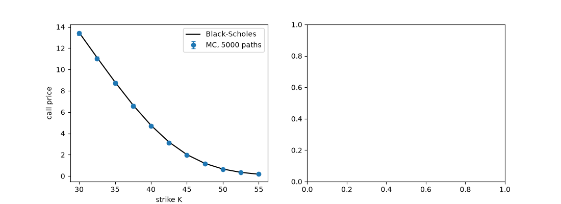
Prices across strikes, with 95% intervals

strikes = np.linspace(30, 55, 11)
mc = [european_option_mc(S, k, T, r, sigma, n_paths=5000, rng=1) for k in strikes]
fig, axes = plt.subplots(1, 2, figsize=(11, 4))
axes[0].plot(strikes, black_scholes_price(S, strikes, T, r, sigma), "k", label="Black-Scholes")
axes[0].errorbar(strikes, [m.estimate for m in mc], yerr=[m.half_width for m in mc], fmt="o", capsize=3, label="MC, 5000 paths")
axes[0].set_xlabel("strike K")
axes[0].set_ylabel("call price")
axes[0].legend()

<matplotlib.legend.Legend object at 0x11207dbe0>

The standard error halves when the paths quadruple

ns = 1000 * 4 ** np.arange(5)
se = [european_option_mc(S, K, T, r, sigma, n_paths=n, rng=2).std_error for n in ns]
plot_error_convergence(ns, se, ax=axes[1], label="standard error")
fig.tight_layout()
plt.show()