Paskov-Traub: QMC in high dimension

Theory said quasi-Monte Carlo should lose its edge beyond a dozen dimensions, since \((\log N)^d / N\) only beats \(N^{-1/2}\) for astronomically large \(N\). Spassimir Paskov and Joseph Traub (1995) priced a Goldman Sachs collateralized mortgage obligation, a 360-dimensional integral, and found Sobol points beat Monte Carlo anyway. The explanation, later formalized as effective dimension: financial integrands depend mostly on a few coordinates and their low-order interactions.

Here: a discretely monitored arithmetic Asian call on 64 dates, a 64-dimensional integral, with Sobol increments driving the steps in time order (financialkit.integrators.sobol_increments() with bridge=False).

import matplotlib.pyplot as plt
import numpy as np

from financialkit.integrators import gbm_paths
from financialkit.monte_carlo import gbm_path_estimate
from financialkit.monte_carlo.visualizers import plot_error_convergence

S, K, T, r, sigma, d = 100.0, 100.0, 1.0, 0.05, 0.2, 64


def asian(paths):
    return np.maximum(paths[:, 1:].mean(axis=1) - K, 0.0)

Standard error against paths

Both estimates are replicated eight times with fresh seeds; the standard errors are on the same footing.

ns = 2 ** np.arange(7, 12)
results = {s: [gbm_path_estimate(asian, S, T, r, sigma, d, n, sampler=s, n_replications=8, rng=n) for n in ns] for s in ("pseudo", "sobol")}
fig, axes = plt.subplots(1, 2, figsize=(12, 4))
plot_error_convergence(ns, [x.std_error for x in results["pseudo"]], ax=axes[0], label="Monte Carlo", rates=(0.5,))
plot_error_convergence(ns, [x.std_error for x in results["sobol"]], ax=axes[0], label="Sobol, 64 dimensions", rates=())
axes[0].set_title("arithmetic Asian call, 64 dates")
for s in ("pseudo", "sobol"):
    x = results[s][-1]
    print(f"{s:7s}: {x.estimate:.4f} +/- {x.std_error:.4f}")

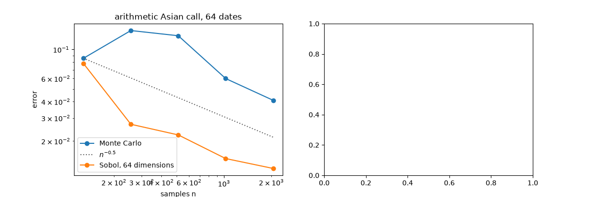
pseudo : 5.8934 +/- 0.0410
sobol  : 5.8454 +/- 0.0124

The integrand’s effective dimension is low

Payoff sensitivity to each Sobol coordinate, by perturbing one normal at a time: the average depends on every increment, but those of the early dates matter most, since they move more of the average.

z = np.random.default_rng(0).standard_normal((4000, d))
base = asian(gbm_paths(S, r, sigma, T, d, 4000, dW=np.sqrt(T / d) * z)[1])
sens = []
for i in range(d):
    zi = z.copy()
    zi[:, i] += 0.1
    sens.append(np.mean(np.abs(asian(gbm_paths(S, r, sigma, T, d, 4000, dW=np.sqrt(T / d) * zi)[1]) - base)))
axes[1].bar(np.arange(1, d + 1), sens)
axes[1].set_xlabel("coordinate (time step)")
axes[1].set_ylabel("mean |payoff change|")
fig.tight_layout()
plt.show()