Caflisch-Moskowitz Brownian bridge

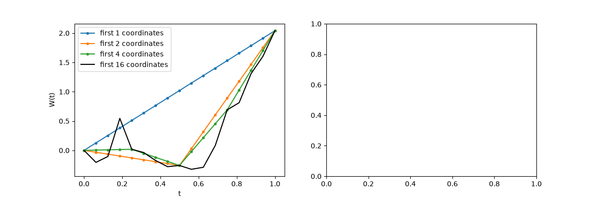
Quasi-random points are best distributed in their first coordinates. If those coordinates drive the first time steps, the coarse shape of each path is left to the poorly distributed later ones. Russel Caflisch and Bradley Moskowitz (1995), and Caflisch, Morokoff and Owen (1997) for mortgage-backed securities, reordered the construction: the first coordinate sets \(W(T)\), the second \(W(T/2)\) given the ends, and so on by bisection,

\[W(t_m) \mid W(t_l), W(t_r) \sim N\left(\frac{(t_r - t_m)W(t_l) + (t_m - t_l)W(t_r)}{t_r - t_l},\; \frac{(t_m - t_l)(t_r - t_m)}{t_r - t_l}\right),\]

which concentrates the variance in the leading coordinates and lowers the effective dimension.

import matplotlib.pyplot as plt
import numpy as np

from financialkit.integrators import brownian_bridge
from financialkit.monte_carlo import gbm_path_estimate
from financialkit.monte_carlo.visualizers import plot_error_convergence

Coarse shape first

The same normals, used in bridge order: after 1, 2 and 4 coordinates the path’s outline is already in place.

z = np.random.default_rng(3).standard_normal(16)
fig, axes = plt.subplots(1, 2, figsize=(12, 4))
t = np.linspace(0, 1, 17)
for k in (1, 2, 4, 16):
    zk = np.where(np.arange(16) < k, z, 0.0)
    axes[0].plot(t, brownian_bridge(zk[None, :], 1.0)[0], "o-" if k < 16 else "k-", ms=3, label=f"first {k} coordinates")
axes[0].set_xlabel("t")
axes[0].set_ylabel("W(t)")
axes[0].legend()

<matplotlib.legend.Legend object at 0x111efdd30>

Bridge Sobol against time-ordered Sobol

The 64-date Asian call of the Paskov-Traub example.

S, K, T, r, sigma, d = 100.0, 100.0, 1.0, 0.05, 0.2, 64


def asian(paths):
    return np.maximum(paths[:, 1:].mean(axis=1) - K, 0.0)


ns = 2 ** np.arange(7, 12)
for s, label in [("pseudo", "Monte Carlo"), ("sobol", "Sobol, time order"), ("bridge", "Sobol, Brownian bridge")]:
    res = [gbm_path_estimate(asian, S, T, r, sigma, d, n, sampler=s, n_replications=8, rng=n) for n in ns]
    plot_error_convergence(ns, [x.std_error for x in res], ax=axes[1], label=label, rates=(0.5,) if s == "pseudo" else ())
    print(f"{label:24s}: {res[-1].estimate:.4f} +/- {res[-1].std_error:.5f}")
fig.tight_layout()
plt.show()

Monte Carlo             : 5.8934 +/- 0.04095
Sobol, time order       : 5.8454 +/- 0.01236
Sobol, Brownian bridge  : 5.8393 +/- 0.00283