Neyman stratification

Jerzy Neyman (1934) showed survey statisticians how to sample a stratified population: draw from each stratum separately and allocate the sample in proportion to the stratum’s weight times its standard deviation,

\[n_h \propto p_h \sigma_h, \qquad \operatorname{Var}\hat\mu = \sum_h \frac{p_h^2 \sigma_h^2}{n_h}.\]

In Monte Carlo the “population” is the unit interval that drives the terminal stock price through \(Z = \Phi^{-1}(U)\). Equal-probability strata of \(U\) remove the between-strata variance, and Neyman’s allocation puts the remaining samples where the payoff varies most: in the money.

import matplotlib.pyplot as plt
import numpy as np
from scipy.stats import norm

from financialkit.monte_carlo import european_option_mc, stratified_estimate, terminal_prices, vanilla_payoff
from financialkit.monte_carlo.visualizers import plot_allocation, plot_estimator_comparison
from financialkit.options import black_scholes_price

S, K, T, r, sigma = 100.0, 110.0, 1.0, 0.05, 0.2
exact = black_scholes_price(S, K, T, r, sigma)


def call(u):
    return np.exp(-r * T) * vanilla_payoff(terminal_prices(S, T, r, sigma, norm.ppf(u)), K)

Crude, proportional and Neyman allocations

n = 10_000
crude = european_option_mc(S, K, T, r, sigma, n_paths=n, rng=0)
prop = stratified_estimate(call, n, n_strata=20, allocation="proportional", rng=1)
ney = stratified_estimate(call, n, n_strata=20, allocation="neyman", rng=2)
for res in (crude, prop, ney):
    print(f"{res.method:24s} {res.estimate:.4f} +/- {res.std_error:.4f}  variance reduction x{res.variance_ratio(crude):.1f}")

fig, axes = plt.subplots(1, 2, figsize=(12, 4))
plot_estimator_comparison([crude, prop, ney], exact=exact, ax=axes[0])

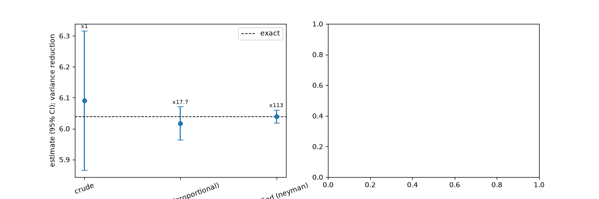
crude                    6.0910 +/- 0.1148  variance reduction x1.0
stratified (proportional) 6.0174 +/- 0.0273  variance reduction x17.7
stratified (neyman)      6.0396 +/- 0.0107  variance reduction x113.0

<Axes: ylabel='estimate (95% CI); variance reduction'>

Where Neyman puts the samples

Strata of low \(U\) end out of the money with zero variance and get only the two-sample floor.

plot_allocation(ney, ax=axes[1])
fig.tight_layout()
plt.show()