Lavenberg-Welch control variates

If a quantity \(X\) simulated alongside the target \(Y\) has a known mean, its sampling error tells us about the error in \(\bar Y\). Stephen Lavenberg and Peter Welch (1981) framed the correction as a regression: estimate \(\beta\) by least squares and use

\[\hat\mu = \bar Y - \beta^\top(\bar X - \mu_X), \qquad \operatorname{Var}\hat\mu \approx (1 - R^2)\frac{s_Y^2}{n}.\]

The discounted terminal stock price, with mean \(S e^{-qT}\), is the natural control for a call; the closer to the money, the better it explains the payoff.

import matplotlib.pyplot as plt
import numpy as np

from financialkit.monte_carlo import control_variate_estimate, terminal_prices, vanilla_payoff
from financialkit.options import black_scholes_price

S, T, r, sigma = 100.0, 1.0, 0.05, 0.2
z = np.random.default_rng(0).standard_normal(10_000)
S_T = terminal_prices(S, T, r, sigma, z)
X = np.exp(-r * T) * S_T

The regression behind the estimator

K = 90.0
Y = np.exp(-r * T) * vanilla_payoff(S_T, K)
res = control_variate_estimate(Y, X, S)
print(f"K = {K}: crude {res.crude_estimate:.4f} +/- {res.crude_std_error:.4f}, controlled {res.estimate:.4f} +/- {res.std_error:.4f}")
print(f"Black-Scholes {black_scholes_price(S, K, T, r, sigma):.4f}, beta {res.beta[0]:.3f}, R^2 {res.r_squared:.3f}")

fig, axes = plt.subplots(1, 2, figsize=(12, 4))
axes[0].scatter(X[:2000], Y[:2000], s=2, alpha=0.4)
xs = np.linspace(X.min(), X.max(), 2)
axes[0].plot(xs, Y.mean() + res.beta[0] * (xs - X.mean()), "k", label=rf"$\beta = {res.beta[0]:.2f}$")
axes[0].set_xlabel(r"control $e^{-rT} S_T$")
axes[0].set_ylabel("discounted payoff")
axes[0].legend()

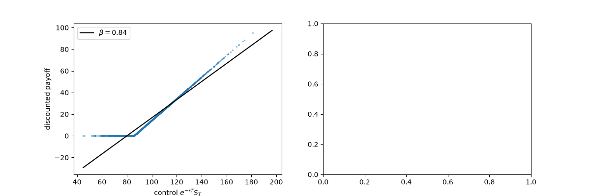
K = 90.0: crude 16.7734 +/- 0.1731, controlled 16.6782 +/- 0.0418
Black-Scholes 16.6994, beta 0.835, R^2 0.942

<matplotlib.legend.Legend object at 0x111f73a10>

The gain across strikes, with one and two controls

Adding the discounted at-the-money call as a second control (its Black-Scholes price is known) helps the out-of-the-money strikes.

strikes = np.linspace(70, 140, 15)
atm = np.exp(-r * T) * vanilla_payoff(S_T, 100.0)
controls = np.column_stack([X, atm])
means = [S, black_scholes_price(S, 100.0, T, r, sigma)]
one = [1 / (1 - control_variate_estimate(np.exp(-r * T) * vanilla_payoff(S_T, k), X, S).r_squared) for k in strikes]
two = [1 / (1 - min(control_variate_estimate(np.exp(-r * T) * vanilla_payoff(S_T, k), controls, means).r_squared, 1 - 1e-6)) for k in strikes]
axes[1].semilogy(strikes, one, "o-", label=r"control $S_T$")
axes[1].semilogy(strikes, two, "s-", label=r"controls $S_T$ and ATM call")
axes[1].set_xlabel("strike K")
axes[1].set_ylabel(r"variance reduction $1/(1 - R^2)$")
axes[1].legend()
fig.tight_layout()
plt.show()