McKay-Beckman-Conover Latin hypercube

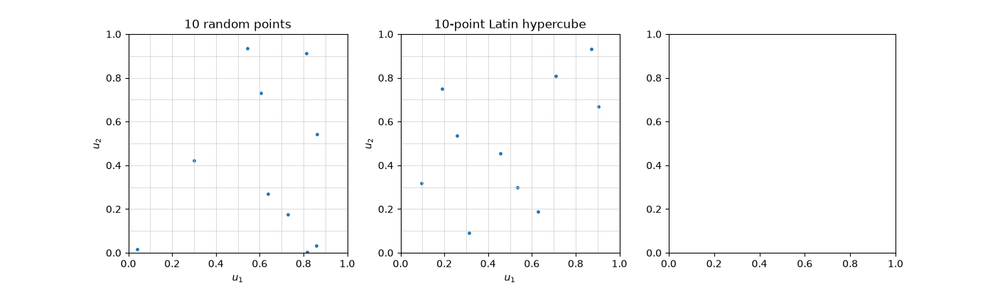
Michael McKay, Richard Beckman and William Conover (1979), at Los Alamos, needed to run expensive computer codes on few input combinations. A Latin hypercube design of \(n\) points stratifies every coordinate into \(n\) equal intervals at once: each interval of each axis holds exactly one point, the axes shuffled independently. The variance of an additive integrand falls by an order of \(n\); interactions are left alone.

import matplotlib.pyplot as plt
import numpy as np
from scipy.stats import norm

from financialkit.monte_carlo import latin_hypercube_estimate, monte_carlo_integrate
from financialkit.monte_carlo.utils import qmc_engine
from financialkit.monte_carlo.visualizers import plot_point_set

One point per row and per column

fig, axes = plt.subplots(1, 3, figsize=(14, 4))
plot_point_set(np.random.default_rng(0).random((10, 2)), ax=axes[0], grid=10, title="10 random points")
plot_point_set(qmc_engine("lhs", 2, rng=0).random(10), ax=axes[1], grid=10, title="10-point Latin hypercube")

<Axes: title={'center': '10-point Latin hypercube'}, xlabel='$u_{1}$', ylabel='$u_{2}$'>

A basket of five lognormal assets

The basket’s mean value is nearly additive in the inputs; a call on it is less so. Both gain, the additive one far more.

d, n = 5, 500
basket = lambda u: np.mean(np.exp(0.2 * norm.ppf(u) - 0.02), axis=1)  # noqa: E731
call = lambda u: np.maximum(basket(u) - 1.0, 0.0)  # noqa: E731
labels, ratios = [], []
for name, f in [("basket mean", basket), ("basket call", call)]:
    crude = monte_carlo_integrate(f, 20 * n, dim=d, rng=1)
    lhs = latin_hypercube_estimate(f, n, d, n_replications=20, rng=2)
    print(f"{name}: crude {crude.estimate:.5f} +/- {crude.std_error:.5f}, LHS {lhs.estimate:.5f} +/- {lhs.std_error:.5f}")
    labels.append(name)
    ratios.append(lhs.variance_ratio(crude))
axes[2].bar(labels, ratios)
axes[2].set_yscale("log")
axes[2].set_ylabel("variance reduction factor")
axes[2].set_title(f"LHS, n = {n}, d = {d}")
fig.tight_layout()
plt.show()

basket mean: crude 0.99987 +/- 0.00092, LHS 0.99999 +/- 0.00002
basket call: crude 0.03652 +/- 0.00056, LHS 0.03573 +/- 0.00021