Bachelier’s normal model

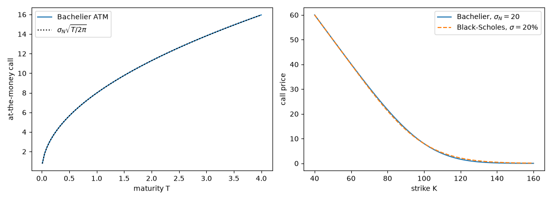
In his 1900 thesis Théorie de la spéculation Louis Bachelier modelled the price of a French government bond as a Brownian motion and priced options on it, five years before Einstein’s paper on Brownian motion. In his model price changes are normal with an absolute volatility \(\sigma_N\), so an at-the-money option is worth \(\sigma_N\sqrt{T/(2\pi)}\): the square-root-of-time law. Below, the formula is checked against simulated arithmetic Brownian paths and compared with Black-Scholes at a matched volatility.

import matplotlib.pyplot as plt
import numpy as np

from financialkit.options import bachelier_price, black_scholes_price

Monte Carlo under arithmetic Brownian motion

S0, T, sigma_n = 100.0, 1.0, 20.0
rng = np.random.default_rng(0)
S_T = S0 + sigma_n * np.sqrt(T) * rng.standard_normal(200_000)
for K in (90.0, 100.0, 110.0):
    payoff = np.maximum(S_T - K, 0.0)
    mc, se = payoff.mean(), payoff.std() / np.sqrt(payoff.size)
    print(f"K = {K:5.1f}: Bachelier {bachelier_price(S0, K, T, 0.0, sigma_n):.4f}, Monte Carlo {mc:.4f} +/- {1.96 * se:.4f}")

K =  90.0: Bachelier 13.9559, Monte Carlo 13.9691 +/- 0.0652
K = 100.0: Bachelier 7.9788, Monte Carlo 7.9905 +/- 0.0512
K = 110.0: Bachelier 3.9559, Monte Carlo 3.9597 +/- 0.0362

The square-root-of-time law, and the comparison with Black-Scholes

With \(\sigma_N = \sigma S_0\) the two models nearly agree near the money for short maturities; Bachelier’s prices go negative only in the far tail of the normal, which lognormal Black-Scholes never does.

maturities = np.linspace(0.01, 4.0, 100)
K = np.linspace(40, 160, 121)
fig, axes = plt.subplots(1, 2, figsize=(11, 4))
axes[0].plot(maturities, bachelier_price(S0, S0, maturities, 0.0, sigma_n), label="Bachelier ATM")
axes[0].plot(maturities, sigma_n * np.sqrt(maturities / (2 * np.pi)), "k:", label=r"$\sigma_N\sqrt{T/2\pi}$")
axes[0].set_xlabel("maturity T")
axes[0].set_ylabel("at-the-money call")
axes[0].legend()
axes[1].plot(K, bachelier_price(S0, K, T, 0.0, sigma_n), label="Bachelier, $\\sigma_N = 20$")
axes[1].plot(K, black_scholes_price(S0, K, T, 0.0, 0.2), "--", label="Black-Scholes, $\\sigma = 20\\%$")
axes[1].set_xlabel("strike K")
axes[1].set_ylabel("call price")
axes[1].legend()
fig.tight_layout()

plt.show()