Merton: dividends and no-arbitrage bounds

Robert Merton’s Theory of Rational Option Pricing (1973) did two things at once. It derived, with no model, the bounds every European option price must respect,

\[\max(S e^{-qT} - K e^{-rT}, 0) \le c \le S e^{-qT},\]

and it extended Black-Scholes to a stock paying a continuous dividend yield \(q\), which simply replaces \(S\) by \(S e^{-qT}\).

import matplotlib.pyplot as plt
import numpy as np

from financialkit.options import black_scholes_price, no_arbitrage_bounds

Hull’s index option (Example 17.1)

price = black_scholes_price(930.0, 900.0, 2 / 12, 0.08, 0.20, q=0.03)
print(f"two-month call on an index yielding 3%: {price:.2f} (Hull: 51.83)")

two-month call on an index yielding 3%: 51.83 (Hull: 51.83)

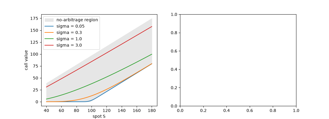
Every Black-Scholes price lies inside Merton’s bounds

As volatility goes to zero the price falls to the lower bound; as it grows without limit the call becomes worth the (dividend-adjusted) stock itself.

S = np.linspace(40, 180, 141)
K, T, r, q = 100.0, 1.0, 0.05, 0.03
lo, hi = no_arbitrage_bounds(S, K, T, r, q)
fig, axes = plt.subplots(1, 2, figsize=(11, 4))
axes[0].fill_between(S, lo, hi, color="0.9", label="no-arbitrage region")
for sigma in (0.05, 0.3, 1.0, 3.0):
    axes[0].plot(S, black_scholes_price(S, K, T, r, sigma, q), label=f"sigma = {sigma}")
axes[0].set_xlabel("spot S")
axes[0].set_ylabel("call value")
axes[0].legend()

<matplotlib.legend.Legend object at 0x116634ec0>

Dividends lower calls and raise puts

yields = np.linspace(0.0, 0.10, 41)
axes[1].plot(yields, black_scholes_price(100.0, K, T, r, 0.25, yields), label="call")
axes[1].plot(yields, black_scholes_price(100.0, K, T, r, 0.25, yields, option_type="put"), label="put")
axes[1].set_xlabel("dividend yield q")
axes[1].set_ylabel("at-the-money value")
axes[1].legend()
fig.tight_layout()

plt.show()