Black-76: options on futures

Fischer Black (1976) priced options on commodity futures. A futures contract costs nothing to enter, so its risk-neutral drift is zero and the Black-Scholes argument gives

\[c = e^{-rT}[F N(d_1) - K N(d_2)],\]

with the futures price \(F\) in place of the spot. The same formula prices caps, floors and swaptions in financialkit.interest_rate_models.

import matplotlib.pyplot as plt
import numpy as np

from financialkit.options import black76_price, black_scholes_price

Hull’s futures put (Example 18.7)

print(f"four-month put on futures at 20, strike 20: {black76_price(20.0, 20.0, 4 / 12, 0.09, 0.25, 'put'):.4f} (Hull: 1.12)")

four-month put on futures at 20, strike 20: 1.1166 (Hull: 1.12)

Black-76 is Black-Scholes on the forward

For a stock with dividend yield \(q\) the forward is \(F = S e^{(r-q)T}\), and both formulas give the same price.

S, T, r, q, sigma = 100.0, 1.0, 0.05, 0.02, 0.25
F = S * np.exp((r - q) * T)
K = np.linspace(70, 140, 8)
print("max difference:", np.max(np.abs(black76_price(F, K, T, r, sigma) - black_scholes_price(S, K, T, r, sigma, q))))

max difference: 0.0

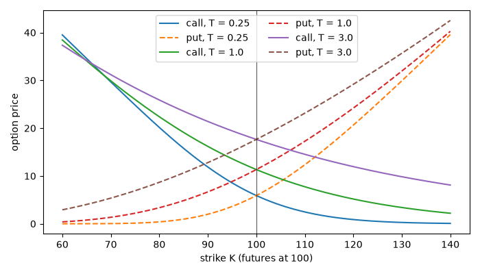
Calls and puts on futures across maturities

K = np.linspace(60, 140, 161)
fig, ax = plt.subplots(figsize=(7, 4))
for T in (0.25, 1.0, 3.0):
    ax.plot(K, black76_price(100.0, K, T, 0.05, 0.3), label=f"call, T = {T}")
    ax.plot(K, black76_price(100.0, K, T, 0.05, 0.3, "put"), "--", label=f"put, T = {T}")
ax.axvline(100.0, color="k", lw=0.5)
ax.set_xlabel("strike K (futures at 100)")
ax.set_ylabel("option price")
ax.legend(ncol=2)
fig.tight_layout()

plt.show()