Garman-Kohlhagen currency options

Mark Garman and Steven Kohlhagen (1983) noticed that a unit of foreign currency is an asset that pays the foreign interest rate \(r_f\), just as a stock pays a dividend yield. Merton’s dividend formula then prices FX options:

\[c = S e^{-r_f T} N(d_1) - K e^{-r_d T} N(d_2).\]

A call on one currency is a put on the other, which gives a symmetry check.

import matplotlib.pyplot as plt
import numpy as np

from financialkit.options import garman_kohlhagen_price

Haug’s example

price = garman_kohlhagen_price(1.56, 1.60, 0.5, 0.06, 0.08, 0.12)
print(f"six-month call, S = 1.56, K = 1.60, r_d = 6%, r_f = 8%: {price:.4f} (Haug: 0.0291)")

six-month call, S = 1.56, K = 1.60, r_d = 6%, r_f = 8%: 0.0291 (Haug: 0.0291)

Foreign-domestic symmetry

A call to buy one unit of foreign currency at \(K\) equals \(S K\) times a put, in foreign units, to sell one unit of domestic currency at \(1/K\), with the rates swapped and the spot inverted.

S, K, T, rd, rf, sigma = 1.56, 1.60, 0.5, 0.06, 0.08, 0.12
call = garman_kohlhagen_price(S, K, T, rd, rf, sigma)
put_inverse = garman_kohlhagen_price(1 / S, 1 / K, T, rf, rd, sigma, "put")
print(f"call {call:.6f} = S K x inverse put {S * K * put_inverse:.6f}")

call 0.029099 = S K x inverse put 0.029099

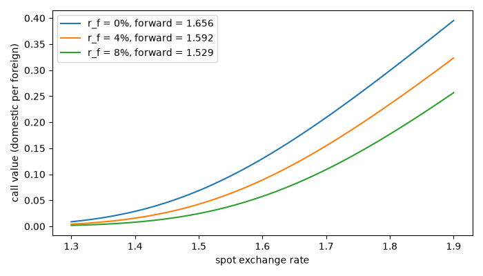
The interest-rate differential shifts the forward

spots = np.linspace(1.3, 1.9, 121)
fig, ax = plt.subplots(figsize=(7, 4))
for rf in (0.0, 0.04, 0.08):
    ax.plot(spots, garman_kohlhagen_price(spots, K, 1.0, 0.06, rf, sigma), label=f"r_f = {rf:.0%}, forward = {1.56 * np.exp(0.06 - rf):.3f}")
ax.set_xlabel("spot exchange rate")
ax.set_ylabel("call value (domestic per foreign)")
ax.legend()
fig.tight_layout()

plt.show()