Latané-Rendleman implied volatility

Every input to Black-Scholes is observable except the volatility. Henry Latané and Richard Rendleman (1976) turned the formula around: given a market price, solve for the volatility that reproduces it. The price is strictly increasing in \(\sigma\) between Merton’s bounds, so the root is unique; it exists only for prices strictly inside them.

import matplotlib.pyplot as plt
import numpy as np

from financialkit.options import black_scholes_price, implied_volatility, no_arbitrage_bounds

Hull’s example (Section 15.11)

print(f"implied vol of a 1.875 call (S = 21, K = 20, r = 10%, 3 months): {implied_volatility(1.875, 21.0, 20.0, 0.25, 0.10):.4f}")

implied vol of a 1.875 call (S = 21, K = 20, r = 10%, 3 months): 0.2345

The price is monotone in volatility, so the inverse is unique

S, K, T, r = 100.0, 110.0, 0.5, 0.03
sigmas = np.linspace(0.001, 2.0, 400)
prices = black_scholes_price(S, K, T, r, sigmas)
lo, hi = no_arbitrage_bounds(S, K, T, r)
target = 4.0
iv = implied_volatility(target, S, K, T, r)
print(f"a {target} call has implied volatility {iv:.4f}")

fig, ax = plt.subplots(figsize=(7, 4))
ax.plot(sigmas, prices, label="Black-Scholes price")
ax.axhline(lo, color="k", ls=":", label="Merton bounds")
ax.axhline(hi, color="k", ls=":")
ax.plot([0, iv, iv], [target, target, 0], "r--", lw=1)
ax.plot(iv, target, "ro", label=f"implied vol = {iv:.3f}")
ax.set_xlabel("volatility")
ax.set_ylabel("call price")
ax.set_ylim(0, 60)
ax.legend()
fig.tight_layout()

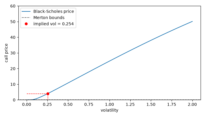
a 4.0 call has implied volatility 0.2538

Prices outside the bounds have no implied volatility

try:
    implied_volatility(0.5 * lo, S, 80.0, T, r)
except ValueError as err:
    print("ValueError:", err)

plt.show()

ValueError: price 0 violates the no-arbitrage bounds (21.191, 100); no implied volatility exists