Breeden-Litzenberger risk-neutral density

Douglas Breeden and Robert Litzenberger (1978) showed that the second strike derivative of the call price is the discounted risk-neutral density of the terminal price,

\[f(K) = e^{rT} \frac{\partial^2 c}{\partial K^2}.\]

A butterfly spread around \(K\) pays off only if \(S_T\) lands near \(K\), so its price is the market’s state price for that outcome. Black-Scholes prices give back the lognormal; prices from a two-regime mixture reveal a bimodal market view.

import matplotlib.pyplot as plt
import numpy as np
from scipy.integrate import trapezoid
from scipy.stats import lognorm

from financialkit.options import black_scholes_price, breeden_litzenberger_density
from financialkit.options.visualizers import plot_density

Black-Scholes prices recover the lognormal density

S, T, r, sigma = 100.0, 0.5, 0.03, 0.25
K = np.linspace(30, 220, 381)
res = breeden_litzenberger_density(K, black_scholes_price(S, K, T, r, sigma), T, r)
exact = lognorm.pdf(res.strikes, s=sigma * np.sqrt(T), scale=S * np.exp((r - 0.5 * sigma**2) * T))
print(f"max error against the lognormal: {np.max(np.abs(res.density - exact)):.1e}")

fig, axes = plt.subplots(1, 2, figsize=(11, 4))
plot_density(res, ax=axes[0])
axes[0].plot(res.strikes, exact, "k:", label="lognormal")
axes[0].legend()

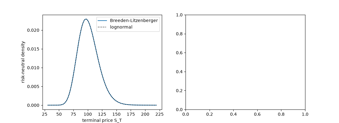
max error against the lognormal: 1.7e-06

<matplotlib.legend.Legend object at 0x1167d17f0>

A bimodal market: an event with two outcomes

Mix two lognormals with forwards 85 and 115, the same overall forward, as before a binary event. The density from the mixed prices shows both modes, which no single Black-Scholes volatility could produce.

w = 0.5
F = S * np.exp(r * T)
mix = w * black_scholes_price(0.85 * S, K, T, r, 0.1) + (1 - w) * black_scholes_price(1.15 * S, K, T, r, 0.1)
res_mix = breeden_litzenberger_density(K, mix, T, r)
plot_density(res_mix, ax=axes[1], label="two-regime prices")
axes[1].axvline(F, color="k", lw=0.5)
print(f"total probability: {trapezoid(res_mix.density, res_mix.strikes):.4f}")
fig.tight_layout()

plt.show()

total probability: 1.0000