The volatility smile

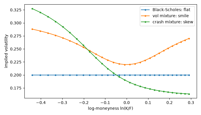
Under Black-Scholes every strike has the same implied volatility. Before October 1987 index options roughly agreed; after the crash, low-strike puts became permanently more expensive, and implied volatility fell steeply with the strike (Rubinstein 1994). Inverting a strip of option prices strike by strike shows the market’s departure from the lognormal. Here the prices come from two simple arbitrage-free models: a mixture of volatilities (a symmetric smile) and a mixture of a normal regime with a crash regime (a skew).

import matplotlib.pyplot as plt
import numpy as np

from financialkit.options import black_scholes_price, implied_vol_smile
from financialkit.options.visualizers import plot_smile

S, T, r = 100.0, 0.5, 0.02
K = np.linspace(65, 135, 29)

Flat: Black-Scholes prices

flat = implied_vol_smile(black_scholes_price(S, K, T, r, 0.2), K, S, T, r)
print("Black-Scholes prices, implied vol range:", np.round([flat.vols.min(), flat.vols.max()], 6))

Black-Scholes prices, implied vol range: [0.2 0.2]

Smile: uncertain volatility

smile_prices = 0.5 * black_scholes_price(S, K, T, r, 0.12) + 0.5 * black_scholes_price(S, K, T, r, 0.32)
smile = implied_vol_smile(smile_prices, K, S, T, r)

Skew: a small chance of a crash

With probability 10% the forward is 25% lower; the other regime’s forward is raised so the overall forward is unchanged.

p_crash, drop = 0.10, 0.25
up = (1 - p_crash * (1 - drop)) / (1 - p_crash)
skew_prices = p_crash * black_scholes_price(S * (1 - drop), K, T, r, 0.3) + (1 - p_crash) * black_scholes_price(S * up, K, T, r, 0.15)
skew = implied_vol_smile(skew_prices, K, S, T, r)

fig, ax = plt.subplots(figsize=(7, 4))
plot_smile(flat, ax=ax, label="Black-Scholes: flat", moneyness=True)
plot_smile(smile, ax=ax, label="vol mixture: smile", moneyness=True)
plot_smile(skew, ax=ax, label="crash mixture: skew", moneyness=True)
fig.tight_layout()

plt.show()