The Brenner-Subrahmanyam approximation

Menachem Brenner and Marti Subrahmanyam (1988) gave traders a pocket-calculator implied volatility. At the money forward,

\[c = S e^{-qT}\left[2N\left(\tfrac{\sigma\sqrt{T}}{2}\right) - 1\right] \approx S e^{-qT} \sigma \sqrt{\frac{T}{2\pi}},\]

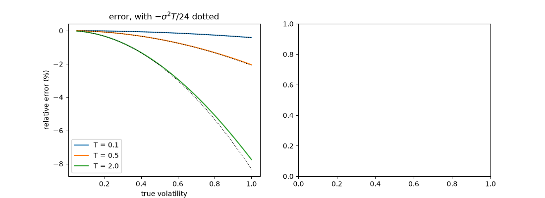
so \(\sigma \approx \sqrt{2\pi/T}\, c / S\), roughly \(2.5\,c/(S\sqrt{T})\). The relative error is about \(-\sigma^2 T / 24\).

import matplotlib.pyplot as plt
import numpy as np

from financialkit.options import black_scholes_price, brenner_subrahmanyam_vol, implied_volatility

A quick estimate against the exact inversion

S, r, T = 100.0, 0.03, 0.5
F = S * np.exp(r * T)
c = black_scholes_price(S, F, T, r, 0.25)
print(f"ATM-forward call {c:.4f}: approximation {brenner_subrahmanyam_vol(c, S, T, r):.5f}, exact {implied_volatility(c, S, F, T, r):.5f}")

ATM-forward call 7.0432: approximation 0.24967, exact 0.25000

Accuracy across volatility and maturity

sigmas = np.linspace(0.05, 1.0, 60)
fig, axes = plt.subplots(1, 2, figsize=(11, 4))
for T in (0.1, 0.5, 2.0):
    F = S * np.exp(r * T)
    approx = brenner_subrahmanyam_vol(black_scholes_price(S, F, T, r, sigmas), S, T, r)
    axes[0].plot(sigmas, 100 * (approx / sigmas - 1), label=f"T = {T}")
    axes[0].plot(sigmas, -100 * sigmas**2 * T / 24, "k:", lw=1)
axes[0].set_xlabel("true volatility")
axes[0].set_ylabel("relative error (%)")
axes[0].set_title(r"error, with $-\sigma^2 T/24$ dotted")
axes[0].legend()

<matplotlib.legend.Legend object at 0x1167d1be0>

Away from the money the approximation breaks down

K = np.linspace(80, 120, 41)
T, sigma = 0.5, 0.25
prices = black_scholes_price(S, K, T, r, sigma)
axes[1].plot(K / (S * np.exp(r * T)), brenner_subrahmanyam_vol(prices, S, T, r), label="Brenner-Subrahmanyam")
axes[1].axhline(sigma, color="k", ls=":", label="true volatility")
axes[1].set_xlabel("moneyness K / F")
axes[1].set_ylabel("estimated volatility")
axes[1].legend()
fig.tight_layout()

plt.show()