The Leisen-Reimer tree

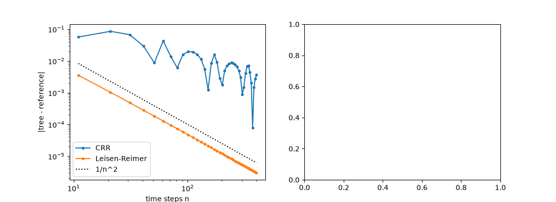
Dietmar Leisen and Matthias Reimer (1996) removed the binomial tree’s oscillation. Instead of fixing \(u\) and \(d\) from the volatility, they choose the probabilities so that the tree’s cumulative binomial distribution reproduces Black-Scholes’s \(N(d_2)\) and \(N(d_1)\), using the Peizer-Pratt inversion of the normal onto the binomial. The tree is centred on the strike, and European prices converge smoothly at order \(1/n^2\).

import matplotlib.pyplot as plt
import numpy as np

from financialkit.options import CRRTree, LeisenReimerTree, black_scholes_price
from financialkit.options.visualizers import plot_tree_convergence

S, K, T, r, sigma = 100.0, 110.0, 1.0, 0.05, 0.25
exact = black_scholes_price(S, K, T, r, sigma)

Second-order convergence

steps = np.arange(11, 402, 10)
crr = [CRRTree(n).price(S, K, T, r, sigma).price for n in steps]
lr = [LeisenReimerTree(n).price(S, K, T, r, sigma).price for n in steps]
order = np.polyfit(np.log(steps), np.log(np.abs(np.array(lr) - exact)), 1)[0]
print(f"Leisen-Reimer empirical order: {-order:.2f}")
err_crr = abs(CRRTree(51).price(S, K, T, r, sigma).price - exact)
err_lr = abs(LeisenReimerTree(51).price(S, K, T, r, sigma).price - exact)
print(f"error with 51 steps: CRR {err_crr:.1e}, Leisen-Reimer {err_lr:.1e}")

fig, axes = plt.subplots(1, 2, figsize=(11, 4))
plot_tree_convergence(steps, crr, exact, ax=axes[0], label="CRR")
plot_tree_convergence(steps, lr, exact, ax=axes[0], label="Leisen-Reimer")
axes[0].loglog(steps, 1.0 / steps**2, "k:", label="1/n^2")
axes[0].legend()

Leisen-Reimer empirical order: 1.98
error with 51 steps: CRR 8.7e-03, Leisen-Reimer 1.8e-04

<matplotlib.legend.Legend object at 0x1166d6270>

American puts converge smoothly too

reference = LeisenReimerTree(2001).price(S, K, T, r, sigma, option_type="put", american=True).price
steps = np.arange(11, 302, 10)
axes[1].plot(steps, [CRRTree(n).price(S, K, T, r, sigma, option_type="put", american=True).price for n in steps], label="CRR")
axes[1].plot(steps, [LeisenReimerTree(n).price(S, K, T, r, sigma, option_type="put", american=True).price for n in steps], label="Leisen-Reimer")
axes[1].axhline(reference, color="k", ls=":", label="LR, 2001 steps")
axes[1].set_xlabel("time steps n")
axes[1].set_ylabel("American put")
axes[1].legend()
fig.tight_layout()

plt.show()