Parkinson’s range volatility

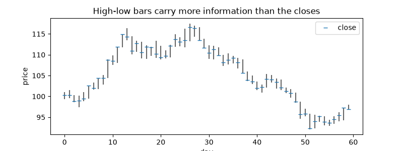
A daily close-to-close return uses two prices out of the thousands traded that day. Michael Parkinson (1980) used two more, the high and the low: for Brownian motion with volatility \(\sigma\),

\[E\bigl[(\ln H_t / L_t)^2\bigr] = 4 \ln 2 \,\sigma^2\,\Delta t,\]

so \((\ln H/L)^2 / (4\ln 2)\) is an unbiased variance estimate whose variance is about 5.2 times smaller than the squared return’s. One month of ranges is as informative as about five months of closes.

import matplotlib.pyplot as plt
import numpy as np

from financialkit.constants import TRADING_DAYS_PER_YEAR
from financialkit.time_series import close_to_close_variance, parkinson_variance
from financialkit.time_series.utils import simulate_ohlc

One year of daily bars

Prices follow a geometric Brownian motion with 25% volatility, sampled every minute of a 390-minute session.

sigma = 0.25
ohlc = simulate_ohlc(1000, sigma, steps_per_day=390, rng=1980)
pk = parkinson_variance(ohlc.high, ohlc.low)
cc = close_to_close_variance(np.r_[ohlc.open[0], ohlc.close])

fig, ax = plt.subplots(figsize=(8, 3))
d = np.arange(60)
ax.vlines(d, ohlc.low[:60], ohlc.high[:60], color="0.4")
ax.plot(d, ohlc.close[:60], "_", color="C0", ms=6, label="close")
ax.set_xlabel("day")
ax.set_ylabel("price")
ax.set_title("High-low bars carry more information than the closes")
ax.legend()

<matplotlib.legend.Legend object at 0x1167fb620>

Rolling 21-day volatility estimates

Both estimators are centred on the true 25%, but the range-based one is far less noisy.

window = 21
kernel = np.ones(window) / window
ann = TRADING_DAYS_PER_YEAR
fig, ax = plt.subplots(figsize=(8, 3.5))
ax.plot(100 * np.sqrt(ann * np.convolve(cc, kernel, "valid")), lw=1, label="close-to-close")
ax.plot(100 * np.sqrt(ann * np.convolve(pk, kernel, "valid")), lw=1, label="Parkinson")
ax.axhline(100 * sigma, color="k", ls="--", lw=1)
ax.set_xlabel("day")
ax.set_ylabel("annualized volatility (%)")
ax.legend()

print(f"mean annualized vol: close-to-close {100 * np.sqrt(ann * cc.mean()):.1f}%, Parkinson {100 * np.sqrt(ann * pk.mean()):.1f}%")
print(f"relative efficiency Var(cc) / Var(Parkinson) = {cc.var() / pk.var():.1f} (theory 5.2)")
plt.show()

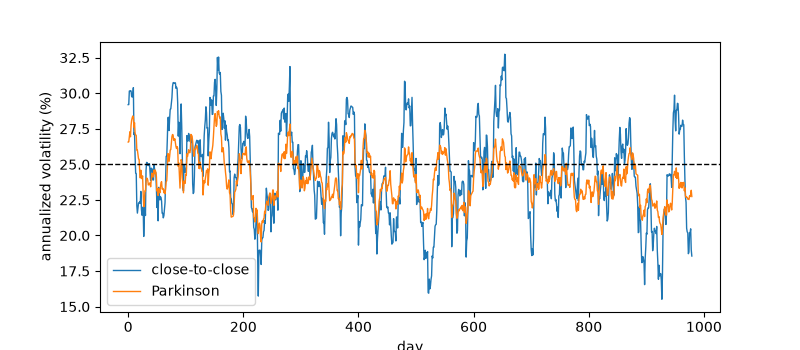
mean annualized vol: close-to-close 24.8%, Parkinson 24.1%
relative efficiency Var(cc) / Var(Parkinson) = 5.0 (theory 5.2)

With one-minute sampling the observed high and low slightly understate the true extremes, which biases the Parkinson estimate down by a few percent; finer sampling removes the bias.