Andersen-Bollerslev realized volatility

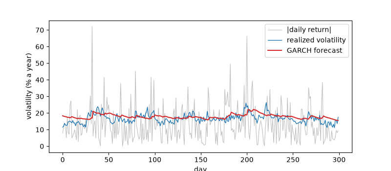
GARCH models fit beautifully in-sample, yet regressions of squared daily returns on their variance forecasts gave \(R^2\) of a few percent, and sceptics concluded the models were useless for forecasting. Torben Andersen and Tim Bollerslev (1998) showed that the fault lay with the yardstick. A squared return \(\sigma_t^2 z_t^2\) is an unbiased but very noisy measure of the day’s variance, and even a perfect forecast explains only a small part of it. Summing squared five-minute returns (realized variance) measures the variance almost exactly, and against it the same forecasts explain many times more.

import matplotlib.pyplot as plt
import numpy as np

from financialkit.constants import TRADING_DAYS_PER_YEAR
from financialkit.time_series import GARCH, mincer_zarnowitz, realized_variance
from financialkit.time_series.utils import simulate_intraday_returns

A GARCH diffusion sampled every five minutes

Daily variances follow a GARCH(1,1); each day’s return is the sum of 78 five-minute returns whose variances add up to that day’s variance.

ann = TRADING_DAYS_PER_YEAR
true = GARCH(omega=0.2**2 / ann * 0.03, alpha=0.1, beta=0.87)
daily_var = true.simulate(2500, rng=1998).variance
intraday = simulate_intraday_returns(daily_var, 78, rng=1)
r = intraday.sum(axis=1)
rv = realized_variance(intraday)

One-step forecasts from a GARCH fitted to the daily returns

forecast = GARCH.fit(r).variance
fig, ax = plt.subplots(figsize=(8, 3.5))
sl = slice(0, 300)
ax.plot(100 * np.sqrt(ann * r[sl] ** 2), color="0.75", lw=0.8, label="|daily return|")
ax.plot(100 * np.sqrt(ann * rv[sl]), color="C0", lw=1, label="realized volatility")
ax.plot(100 * np.sqrt(ann * forecast[sl]), color="C3", lw=1.5, label="GARCH forecast")
ax.set_xlabel("day")
ax.set_ylabel("volatility (% a year)")
ax.legend(loc="upper right")

<matplotlib.legend.Legend object at 0x116d84590>

Mincer-Zarnowitz regressions

The same forecasts, judged against two proxies of the same variance. Even the true variance, a perfect forecast, scores a low \(R^2\) against squared returns.

for name, proxy in (("squared return", r**2), ("realized variance", rv)):
    print(f"perfect forecast vs {name:17s} R^2 = {mincer_zarnowitz(proxy, daily_var).r_squared:.2f}")

fig, axes = plt.subplots(1, 2, figsize=(9, 3.8), sharex=True)
for ax, (name, proxy) in zip(axes, (("squared return", r**2), ("realized variance", rv)), strict=True):
    mz = mincer_zarnowitz(proxy, forecast)
    ax.scatter(1e4 * forecast, 1e4 * proxy, s=3, alpha=0.4)
    f = np.linspace(forecast.min(), forecast.max(), 2)
    ax.plot(1e4 * f, 1e4 * (mz.coef[0] + mz.coef[1] * f), "C3")
    ax.set_title(f"{name}: $R^2$ = {mz.r_squared:.2f}")
    ax.set_xlabel("GARCH forecast (bp$^2$)")
    print(f"{name:17s} a = {1e4 * mz.coef[0]:+.3f} bp^2, b = {mz.coef[1]:.2f}, R^2 = {mz.r_squared:.2f}")
axes[0].set_ylabel("proxy (bp$^2$)")
axes[0].set_yscale("log")
axes[1].set_yscale("log")
fig.tight_layout()
plt.show()

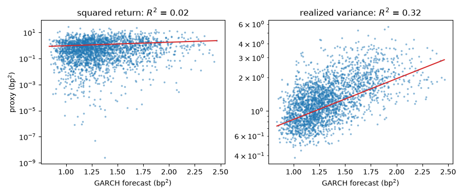
perfect forecast vs squared return    R^2 = 0.07
perfect forecast vs realized variance R^2 = 0.87
squared return    a = +0.094 bp^2, b = 0.93, R^2 = 0.02
realized variance a = -0.367 bp^2, b = 1.32, R^2 = 0.32