Engle’s ARCH

Forecast errors for UK inflation were sometimes small and sometimes large, in clusters. Robert Engle (1982) let the conditional variance depend on the last squared shock,

\[r_t = \sigma_t z_t, \qquad \sigma_t^2 = \omega + \alpha r_{t-1}^2,\]

the autoregressive conditional heteroskedasticity model. Even with normal \(z_t\), the returns are uncorrelated yet dependent, cluster in volatility, and have fat tails (kurtosis \(3(1-\alpha^2)/(1-3\alpha^2)\)). Engle’s Lagrange-multiplier test, \(T R^2\) from regressing \(r_t^2\) on its own lags, detects the effect. The work earned him the 2003 Nobel prize.

import matplotlib.pyplot as plt
import numpy as np

from financialkit.time_series import ARCH, arch_lm_test, autocorrelation, return_statistics
from financialkit.time_series.visualizers import plot_acf, plot_conditional_volatility

Volatility clustering

model = ARCH(omega=0.5, alpha=0.5)
path = model.simulate(4000, rng=1982)
r = path.returns
fig, ax = plt.subplots(figsize=(8, 3.5))
plot_conditional_volatility(r[:500], path.variance[:500], ax=ax)
ax.set_title(r"ARCH(1), $\alpha = 0.5$: calm and turbulent spells")

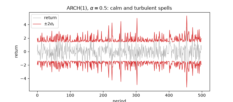
Text(0.5, 1.0, 'ARCH(1), $\\alpha = 0.5$: calm and turbulent spells')

Uncorrelated, but not independent

The returns pass a correlation check; their squares do not. (Sample moments of ARCH returns converge slowly, because for \(\alpha = 0.5\) the eighth moment is infinite, so the sample excess kurtosis understates the theoretical value of 6.)

fig, (ax1, ax2) = plt.subplots(1, 2, figsize=(9, 3.5), sharey=True)
plot_acf(r, 15, ax=ax1)
ax1.set_title("returns")
plot_acf(r**2, 15, ax=ax2)
ax2.set_title("squared returns")
fig.tight_layout()
print(f"lag-1 autocorrelation: returns {autocorrelation(r, 1)[1]:+.2f}, squared returns {autocorrelation(r**2, 1)[1]:+.2f}")
print(f"excess kurtosis {return_statistics(r).excess_kurtosis:.1f}, from normal innovations")

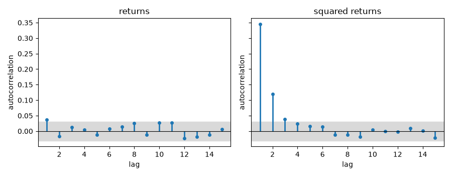
lag-1 autocorrelation: returns +0.04, squared returns +0.35
excess kurtosis 1.3, from normal innovations

The LM test and maximum likelihood

lm = arch_lm_test(r, lags=4)
print(f"ARCH-LM(4) = {lm.statistic:.1f}, p = {lm.pvalue:.2g}")
lm0 = arch_lm_test(np.random.default_rng(0).standard_normal(4000), lags=4)
print(f"on i.i.d. normals: ARCH-LM(4) = {lm0.statistic:.1f}, p = {lm0.pvalue:.2f}")
fit = ARCH.fit(r)
print("MLE:", {k: f"{v:.3f} +/- {fit.std_errors[k]:.3f}" for k, v in fit.params.items()})
plt.show()

ARCH-LM(4) = 476.7, p = 7.2e-102
on i.i.d. normals: ARCH-LM(4) = 8.6, p = 0.07
MLE: {'mu': '-0.002 +/- 0.013', 'omega': '0.530 +/- 0.019', 'alpha': '0.476 +/- 0.032'}