RiskMetrics EWMA

In 1994 J.P. Morgan published RiskMetrics, a free methodology and data set for Value-at-Risk. Its volatility model was deliberately simple: an exponentially weighted moving average

\[\sigma_t^2 = \lambda\,\sigma_{t-1}^2 + (1 - \lambda)\,r_{t-1}^2,\]

with one decay factor for every asset, \(\lambda = 0.94\) for daily and \(0.97\) for monthly data, chosen to minimize forecast errors across hundreds of series. It is GARCH(1,1) with \(\omega = 0\) and \(\alpha + \beta = 1\): no estimation, no long-run level, and a flat term structure of forecasts.

import matplotlib.pyplot as plt
import numpy as np

from financialkit.constants import TRADING_DAYS_PER_YEAR
from financialkit.time_series import EWMA, GARCH

ann = TRADING_DAYS_PER_YEAR

Weights on past squared returns

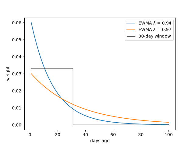
A 0.94 decay puts 6% weight on yesterday and has an effective memory of about 1/(1 - 0.94), roughly 17 days, against an equally weighted window’s hard cut-off.

k = np.arange(1, 101)
fig, ax = plt.subplots()
for lam in (0.94, 0.97):
    ax.plot(k, (1 - lam) * lam ** (k - 1), label=rf"EWMA $\lambda$ = {lam}")
ax.step(k, np.where(k <= 30, 1 / 30, 0.0), where="post", color="k", lw=1, label="30-day window")
ax.set_xlabel("days ago")
ax.set_ylabel("weight")
ax.legend()

<matplotlib.legend.Legend object at 0x116d7dbe0>

Tracking a volatility shock

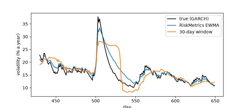
Returns from a GARCH process with a crisis in the middle. EWMA follows the true conditional volatility closely without any fitting; the 30-day window lags it and drops abruptly 30 days after the shock.

g = GARCH(omega=0.15**2 / ann * 0.03, alpha=0.09, beta=0.88)
path = g.simulate(1000, rng=1994)
r = path.returns.copy()
r[500:505] *= 6  # five days of crisis
true_var = g.variance(r, v0=path.variance[0])
ewma = EWMA(0.94).variance(r, v0=path.variance[0])
window = np.convolve(r**2, np.ones(30) / 30)[: r.size]

fig, ax = plt.subplots(figsize=(8, 3.5))
sl = slice(430, 650)
t = np.arange(r.size)[sl]
ax.plot(t, 100 * np.sqrt(ann * true_var[sl]), "k", lw=1.5, label="true (GARCH)")
ax.plot(t, 100 * np.sqrt(ann * ewma[sl]), label="RiskMetrics EWMA")
ax.plot(t, 100 * np.sqrt(ann * window[sl]), label="30-day window")
ax.set_xlabel("day")
ax.set_ylabel("volatility (% a year)")
ax.legend()

<matplotlib.legend.Legend object at 0x116d874d0>

Estimating lambda

Maximum likelihood picks the decay that best fits this one series. RiskMetrics instead fixed 0.94 for every series, trading a little fit for simplicity and comparability across a whole portfolio.

print(f"maximum-likelihood lambda: {EWMA.fit(r).params['lam']:.3f}")
plt.show()

maximum-likelihood lambda: 0.896