Bollerslev’s GARCH

Pure ARCH models needed many lags to capture how slowly volatility decays. Tim Bollerslev (1986), Engle’s student, added the lagged variance itself,

\[\sigma_t^2 = \omega + \alpha\,\varepsilon_{t-1}^2 + \beta\,\sigma_{t-1}^2,\]

an ARCH(\(\infty\)) with geometrically declining weights in three parameters. Fitted to daily returns almost anywhere, GARCH(1,1) gives \(\alpha \approx 0.05\text{-}0.10\) and \(\alpha + \beta\) just below one: shocks to volatility are small but long-lived. Variance forecasts revert to \(\bar\sigma^2 = \omega/(1-\alpha-\beta)\) at rate \((\alpha+\beta)^h\).

import matplotlib.pyplot as plt
import numpy as np

from financialkit.constants import TRADING_DAYS_PER_YEAR
from financialkit.time_series import GARCH
from financialkit.time_series.visualizers import plot_conditional_volatility

Fitting GARCH(1,1) by maximum likelihood

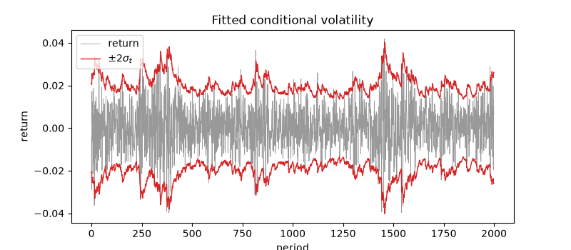
Eight years of daily returns from a GARCH(1,1) with typical equity-index parameters (16% long-run volatility, persistence 0.98).

ann = TRADING_DAYS_PER_YEAR
true = GARCH(omega=0.16**2 / ann * 0.02, alpha=0.08, beta=0.90, mu=3e-4)
r = true.simulate(2000, rng=1986).returns
fit = GARCH.fit(r)
for k, v in fit.params.items():
    print(f"{k:5s} true {true.params[k]:.3g}  fitted {v:.3g} +/- {fit.std_errors[k]:.2g}")
print(f"persistence {fit.model.persistence:.3f}, half-life {fit.model.half_life:.0f} days")

fig, ax = plt.subplots(figsize=(8, 3.5))
plot_conditional_volatility(r, fit.variance, ax=ax)
ax.set_title("Fitted conditional volatility")

mu    true 0.0003  fitted 0.000604 +/- 0.00021
omega true 2.03e-06  fitted 2.44e-06 +/- 8.6e-07
alpha true 0.08  fitted 0.0691 +/- 0.012
beta  true 0.9  fitted 0.908 +/- 0.017
persistence 0.978, half-life 31 days

Text(0.5, 1.0, 'Fitted conditional volatility')

The term structure of volatility forecasts

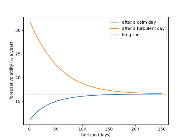
From a calm day and from a turbulent day, forecasts converge to the long-run volatility at the rate set by the persistence.

h = 250
calm = int(np.argmin(fit.variance[500:])) + 500
wild = int(np.argmax(fit.variance[500:])) + 500
fig, ax = plt.subplots()
for name, t in (("after a calm day", calm), ("after a turbulent day", wild)):
    f = fit.model.forecast(r[: t + 1], h)
    ax.plot(np.arange(1, h + 1), 100 * np.sqrt(ann * f), label=name)
ax.axhline(100 * np.sqrt(ann * fit.model.unconditional_variance), color="k", ls="--", lw=1, label="long-run")
ax.set_xlabel("horizon (days)")
ax.set_ylabel("forecast volatility (% a year)")
ax.legend()
plt.show()