Glosten-Jagannathan-Runkle

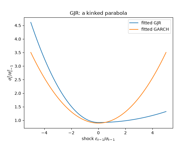
Lawrence Glosten, Ravi Jagannathan and David Runkle (1993) asked whether expected stock returns rise with volatility, and found that the answer depended on modelling volatility’s asymmetric response to news. Their GARCH variant adds one term for negative shocks,

\[\sigma_t^2 = \omega + \bigl(\alpha + \gamma\,\mathbf 1\{\varepsilon_{t-1} < 0\}\bigr)\varepsilon_{t-1}^2 + \beta\,\sigma_{t-1}^2,\]

keeping GARCH’s quadratic shape while letting bad news count \((\alpha + \gamma)/\alpha\) times as much. On U.S. monthly excess returns they found \(\alpha\) near zero: almost all the reaction came from negative shocks.

import matplotlib.pyplot as plt
import numpy as np

from financialkit.time_series import GARCH, GJRGARCH
from financialkit.time_series.visualizers import plot_news_impact

true = GJRGARCH(omega=0.02, alpha=0.01, gamma=0.14, beta=0.91, mu=0.03)

Fitting GJR-GARCH

r = true.simulate(3000, rng=1993).returns
gjr = GJRGARCH.fit(r)
garch = GARCH.fit(r)
for k in ("alpha", "gamma", "beta"):
    print(f"{k:5s} true {true.params[k]:.3f}  fitted {gjr.params[k]:.3f} +/- {gjr.std_errors[k]:.3f}")
print(f"persistence alpha + gamma/2 + beta = {gjr.model.persistence:.3f}")
print(f"likelihood-ratio statistic vs GARCH: {2 * (gjr.loglik - garch.loglik):.1f} (chi^2_1 5% value 3.84)")

ax = plot_news_impact({"fitted GJR": gjr.model, "fitted GARCH": garch.model}, var_prev=true.unconditional_variance)
ax.set_title("GJR: a kinked parabola")

alpha true 0.010  fitted 0.016 +/- 0.009
gamma true 0.140  fitted 0.132 +/- 0.017
beta  true 0.910  fitted 0.909 +/- 0.010
persistence alpha + gamma/2 + beta = 0.991
likelihood-ratio statistic vs GARCH: 68.4 (chi^2_1 5% value 3.84)

Text(0.5, 1.0, 'GJR: a kinked parabola')

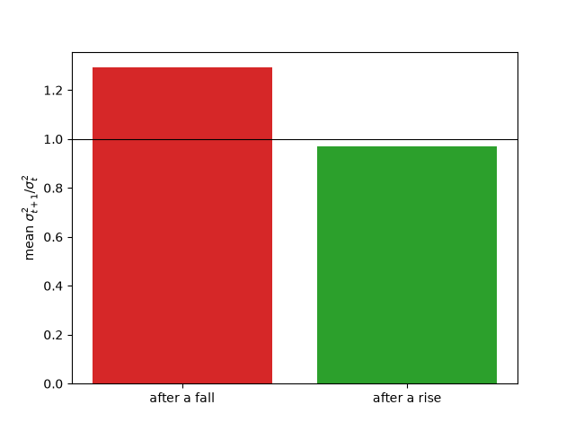
Volatility after up and down days

Average fitted variance the day after a move of more than one standard deviation, by the sign of the move.

z = (r - gjr.model.mean) / np.sqrt(gjr.variance)
nxt = gjr.variance[1:] / gjr.variance[:-1]
fig, ax = plt.subplots()
ax.bar(["after a fall", "after a rise"], [nxt[z[:-1] < -1].mean(), nxt[z[:-1] > 1].mean()], color=["C3", "C2"])
ax.axhline(1, color="k", lw=0.8)
ax.set_ylabel(r"mean $\sigma_{t+1}^2 / \sigma_t^2$")
plt.show()