Nelson’s EGARCH

GARCH reacts to the size of yesterday’s shock but not its sign, and its coefficients must be kept positive. Daniel Nelson (1991) modelled the logarithm of the variance instead,

\[\ln\sigma_t^2 = \omega + \beta\ln\sigma_{t-1}^2 + \alpha\bigl(|z_{t-1}| - E|z|\bigr) + \gamma z_{t-1},\]

which is positive by construction and asymmetric when \(\gamma \ne 0\). For stock returns \(\gamma < 0\): a fall raises volatility more than a rise of the same size, Black’s (1976) “leverage effect”.

import matplotlib.pyplot as plt
import numpy as np

from financialkit.time_series import EGARCH, GARCH
from financialkit.time_series.visualizers import plot_news_impact

The news impact curve

Tomorrow’s variance as a function of today’s standardized shock, starting from the same variance. GARCH’s curve is a symmetric parabola; EGARCH’s is exponential and tilted towards bad news.

egarch = EGARCH(omega=0.0, alpha=0.15, gamma=-0.08, beta=0.97)
garch = GARCH(omega=0.03, alpha=0.08, beta=0.89)
ax = plot_news_impact({"GARCH(1,1)": garch, "EGARCH(1,1)": egarch}, var_prev=1.0)
ax.set_title("News impact: bad news raises EGARCH volatility more")

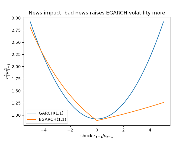
Text(0.5, 1.0, 'News impact: bad news raises EGARCH volatility more')

Estimating the asymmetry

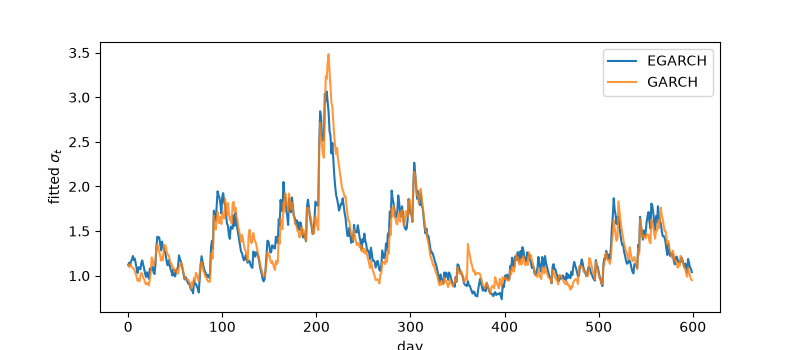
Fitting both models to EGARCH returns: the EGARCH fit recovers a significantly negative \(\gamma\), and its log-likelihood beats GARCH’s with one extra parameter.

r = egarch.simulate(3000, rng=1).returns
eg = EGARCH.fit(r)
ga = GARCH.fit(r)
for k in ("alpha", "gamma", "beta"):
    print(f"{k:5s} true {egarch.params[k]:+.3f}  fitted {eg.params[k]:+.3f} +/- {eg.std_errors[k]:.3f}")
print(f"log-likelihood: EGARCH {eg.loglik:.1f}, GARCH {ga.loglik:.1f}; AIC {eg.aic:.1f} vs {ga.aic:.1f}")

fig, ax = plt.subplots(figsize=(8, 3.5))
ax.plot(np.sqrt(eg.variance[:600]), label="EGARCH")
ax.plot(np.sqrt(ga.variance[:600]), label="GARCH", alpha=0.8)
ax.set_xlabel("day")
ax.set_ylabel(r"fitted $\sigma_t$")
ax.legend()
plt.show()

alpha true +0.150  fitted +0.145 +/- 0.020
gamma true -0.080  fitted -0.083 +/- 0.011
beta  true +0.970  fitted +0.971 +/- 0.006
log-likelihood: EGARCH -4350.1, GARCH -4383.8; AIC 8710.2 vs 8775.5