Witt’s compound-interest tables

Richard Witt’s Arithmeticall Questions (London, 1613) was the first English book of compound-interest tables. For a given rate it listed, year by year, the amount of 1, the present value of 1, and the value of an annuity of 1, so that a clerk could price a loan or a lease with a look-up and a multiplication. This script prints such a table at 10% and uses it to price an annuity.

import matplotlib.pyplot as plt

from financialkit.time_value import annuity_present_value, compound_interest_table

A table at 10%

table = compound_interest_table(0.10, 10)
print(" year   amount of 1   PV of 1   annuity PV   annuity FV")
for k, a, v, an, sn in zip(table.periods, table.amount, table.discount, table.annuity_present, table.annuity_future, strict=True):
    print(f"{k:5d} {a:13.5f} {v:9.5f} {an:12.5f} {sn:12.5f}")

year   amount of 1   PV of 1   annuity PV   annuity FV
   1       1.10000   0.90909      0.90909      1.00000
   2       1.21000   0.82645      1.73554      2.10000
   3       1.33100   0.75131      2.48685      3.31000
   4       1.46410   0.68301      3.16987      4.64100
   5       1.61051   0.62092      3.79079      6.10510
   6       1.77156   0.56447      4.35526      7.71561
   7       1.94872   0.51316      4.86842      9.48717
   8       2.14359   0.46651      5.33493     11.43589
   9       2.35795   0.42410      5.75902     13.57948
  10       2.59374   0.38554      6.14457     15.93742

Using the table

A lease paying 50 a year for 7 years: read a_7 off the table.

print(f"from the table: 50 x {table.annuity_present[6]:.5f} = {50 * table.annuity_present[6]:.2f}")
print(f"direct:         {annuity_present_value(50.0, 0.10, 7):.2f}")

from the table: 50 x 4.86842 = 243.42
direct:         243.42

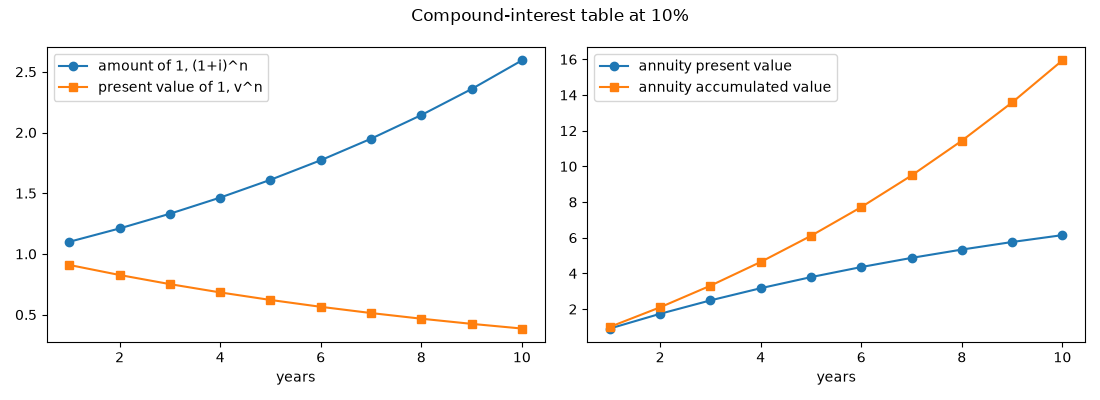
The four columns

fig, axes = plt.subplots(1, 2, figsize=(11, 4))
axes[0].plot(table.periods, table.amount, "o-", label="amount of 1, (1+i)^n")
axes[0].plot(table.periods, table.discount, "s-", label="present value of 1, v^n")
axes[0].set_xlabel("years")
axes[0].legend()
axes[1].plot(table.periods, table.annuity_present, "o-", label="annuity present value")
axes[1].plot(table.periods, table.annuity_future, "s-", label="annuity accumulated value")
axes[1].set_xlabel("years")
axes[1].legend()
fig.suptitle("Compound-interest table at 10%")
fig.tight_layout()

plt.show()