Bernoulli and continuous compounding

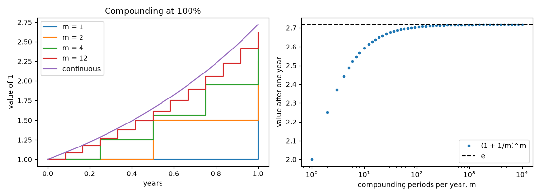
In 1683 Jacob Bernoulli asked what a sum lent at interest becomes if the interest is added not yearly but half-yearly, monthly, daily, at every instant. At 100% a year, 1 grows to \((1 + 1/m)^m\) with m compounding periods, which increases with m but stays bounded; he showed the limit lies between 2.5 and 3. The limit is \(e\), and continuous compounding, \(e^{rt}\), is the convention financialkit uses by default.

import matplotlib.pyplot as plt
import numpy as np

from financialkit.time_value import equivalent_rate, future_value, plot_compounding_growth

Approaching e

for m in (1, 2, 4, 12, 52, 365, 8760):
    print(f"m = {m:5d}: {future_value(1.0, 1.0, 1.0, m):.6f}")
print(f"continuous: {future_value(1.0, 1.0, 1.0):.6f}  (e = {np.e:.6f})")

m =     1: 2.000000
m =     2: 2.250000
m =     4: 2.441406
m =    12: 2.613035
m =    52: 2.692597
m =   365: 2.714567
m =  8760: 2.718127
continuous: 2.718282  (e = 2.718282)

Equivalent rates

The continuously compounded rate giving the same growth as 100% annual interest is ln 2.

print(f"100% annual = {equivalent_rate(1.0, 1, None):.4%} continuous")

100% annual = 69.3147% continuous

Growth paths and the limit

m = np.unique(np.logspace(0, 4, 60).astype(int))
fig, axes = plt.subplots(1, 2, figsize=(11, 4))
plot_compounding_growth(1.0, 1.0, compoundings=(1, 2, 4, 12, None), ax=axes[0])
axes[1].semilogx(m, [future_value(1.0, 1.0, 1.0, int(k)) for k in m], "o", ms=3, label="(1 + 1/m)^m")
axes[1].axhline(np.e, color="k", ls="--", label="e")
axes[1].set_xlabel("compounding periods per year, m")
axes[1].set_ylabel("value after one year")
axes[1].legend()
fig.tight_layout()

plt.show()