Fibonacci’s present value: comparing payment schedules

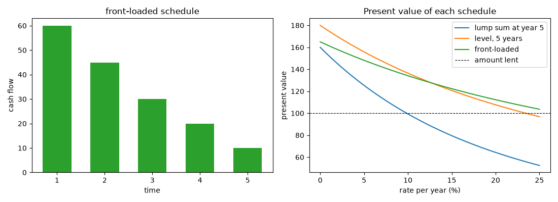
Chapter 12 of Fibonacci’s Liber Abaci (1202) contains problems in which a sum is repaid in instalments at a fixed rate per period, and Fibonacci values each schedule by discounting every instalment back to the start (Goetzmann, 2005). The same idea in modern form: a lender is offered three ways to be repaid a loan of 100 bezants, and the one worth most today depends on the rate. Present value turns each schedule into a single number that can be compared.

import matplotlib.pyplot as plt
import numpy as np

from financialkit.time_value import plot_cash_flows, present_value

Three schedules

Payments in bezants at the end of each year.

schedules = {
    "lump sum at year 5": ([0, 0, 0, 0, 160.0], np.arange(1, 6)),
    "level, 5 years": ([36.0] * 5, np.arange(1, 6)),
    "front-loaded": ([60.0, 45.0, 30.0, 20.0, 10.0], np.arange(1, 6)),
}
for name, (cf, t) in schedules.items():
    pv = present_value(cf, t, 0.10, compounding=1)
    print(f"{name:20s} total {sum(cf):6.1f}  PV at 10% = {pv:6.2f}")

lump sum at year 5   total  160.0  PV at 10% =  99.35
level, 5 years       total  180.0  PV at 10% = 136.47
front-loaded         total  165.0  PV at 10% = 134.14

Which schedule wins depends on the rate

At low rates the larger total wins; at high rates the earlier money wins.

rates = np.linspace(0.0, 0.25, 101)
fig, axes = plt.subplots(1, 2, figsize=(11, 4))
for name, (cf, t) in schedules.items():
    axes[1].plot(100 * rates, present_value(cf, t, rates, compounding=1), label=name)
axes[1].axhline(100.0, color="k", ls="--", lw=0.8, label="amount lent")
axes[1].set_xlabel("rate per year (%)")
axes[1].set_ylabel("present value")
axes[1].set_title("Present value of each schedule")
axes[1].legend()
plot_cash_flows(schedules["front-loaded"][0], schedules["front-loaded"][1], ax=axes[0], title="front-loaded schedule")
fig.tight_layout()

plt.show()