Fisher’s real and nominal rates of interest

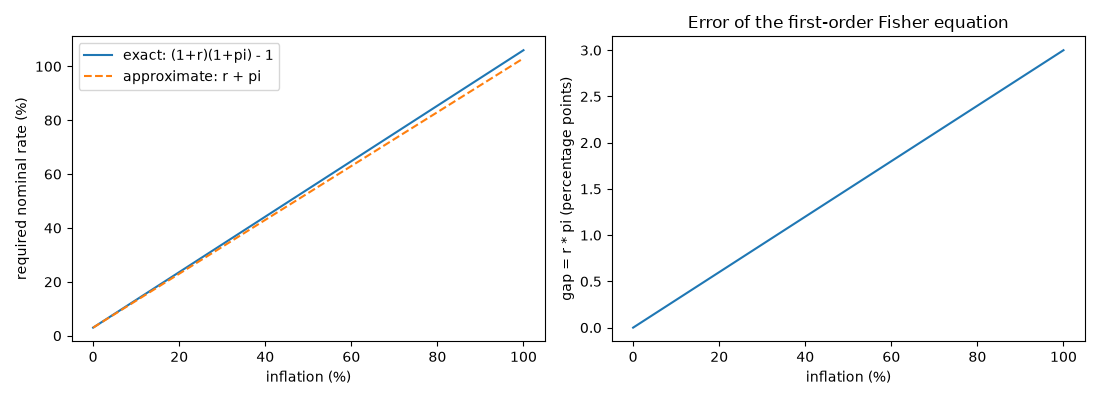
In Appreciation and Interest (1896) Irving Fisher argued that lenders who foresee inflation demand compensation for it, so that a nominal rate \(i\) and a real rate \(r\) satisfy \(1 + i = (1 + r)(1 + \pi)\). The familiar shortcut \(r \approx i - \pi\) is accurate only when inflation is low; this script compares the two across inflation rates, up to hyperinflation.

import matplotlib.pyplot as plt
import numpy as np

from financialkit.time_value import fisher_nominal_rate, fisher_real_rate

A loan at 12% with 8% inflation

print(f"exact real rate:   {fisher_real_rate(0.12, 0.08):.4%}")
print(f"approximate (i-pi): {fisher_real_rate(0.12, 0.08, exact=False):.4%}")
print(f"nominal rate needed for a 3% real return at 8% inflation: {fisher_nominal_rate(0.03, 0.08):.4%}")

exact real rate:   3.7037%
approximate (i-pi): 4.0000%
nominal rate needed for a 3% real return at 8% inflation: 11.2400%

The approximation breaks down as inflation rises

Hold the real rate at 3% and ask what nominal rate a lender needs.

infl = np.linspace(0.0, 1.0, 201)
exact = fisher_nominal_rate(0.03, infl)
approx = 0.03 + infl

fig, axes = plt.subplots(1, 2, figsize=(11, 4))
axes[0].plot(100 * infl, 100 * exact, label="exact: (1+r)(1+pi) - 1")
axes[0].plot(100 * infl, 100 * approx, "--", label="approximate: r + pi")
axes[0].set_xlabel("inflation (%)")
axes[0].set_ylabel("required nominal rate (%)")
axes[0].legend()
axes[1].plot(100 * infl, 100 * (exact - approx))
axes[1].set_xlabel("inflation (%)")
axes[1].set_ylabel("gap = r * pi (percentage points)")
axes[1].set_title("Error of the first-order Fisher equation")
fig.tight_layout()

plt.show()