Fisher’s net present value: choosing between income streams

In The Rate of Interest (1907) Fisher argued that, with access to a capital market, the owner of a firm should choose the income stream with the largest present value at the market rate, whatever their own taste for spending now or later. Net present value is that rule. Here two mutually exclusive projects cost the same; which one has the larger NPV depends on the discount rate, and the profiles cross at Fisher’s “rate of return over cost” between them.

import matplotlib.pyplot as plt
import numpy as np

from financialkit.time_value import irr, npv

Two projects

quick = np.array([-1000.0, 800.0, 300.0, 100.0])
slow = np.array([-1000.0, 300.0, 300.0, 700.0])
for r in (0.05, 0.12):
    print(f"at {r:.0%}: NPV quick = {npv(r, quick):7.2f}, NPV slow = {npv(r, slow):7.2f}")

at 5%: NPV quick =  120.40, NPV slow =  162.51
at 12%: NPV quick =   24.62, NPV slow =    5.26

NPV profiles and the crossover rate

The crossover is the IRR of the difference between the two streams.

crossover = irr(slow - quick)
print(f"crossover rate: {crossover:.4%}")

rates = np.linspace(0.0, 0.30, 121)
fig, ax = plt.subplots(figsize=(7, 4.5))
ax.plot(100 * rates, npv(rates, quick), label="quick payback")
ax.plot(100 * rates, npv(rates, slow), label="slow payback")
ax.axhline(0.0, color="k", lw=0.8)
ax.axvline(100 * crossover, color="gray", ls="--", label=f"crossover {crossover:.1%}")
ax.set_xlabel("discount rate (%)")
ax.set_ylabel("NPV")
ax.set_title("Pick the larger NPV at the market rate")
ax.legend()

plt.show()

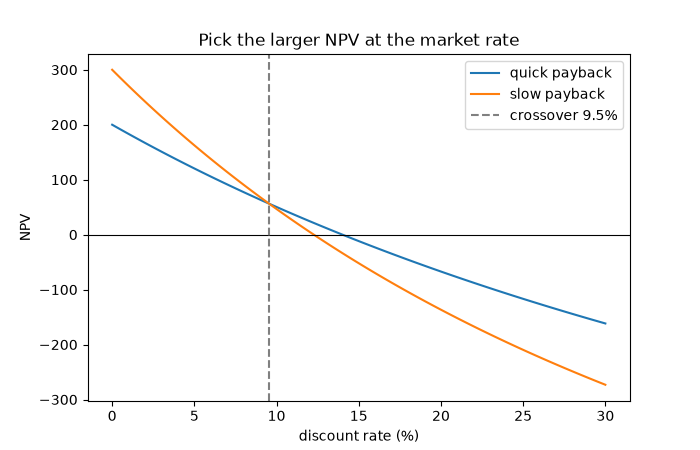
crossover rate: 9.5445%