Clenshaw-Curtis vs. Gauss-Legendre quadrature

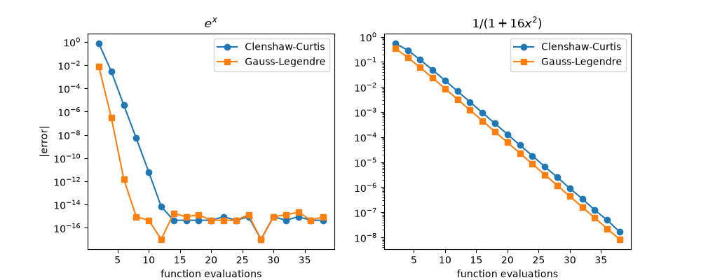
Compares Clenshaw-Curtis quadrature, which integrates the Chebyshev interpolant, with Gauss-Legendre quadrature on smooth integrands. The two converge at nearly the same rate.

import matplotlib.pyplot as plt
import numpy as np

from mathematicskit.calculus import ClenshawCurtisQuadrature, GaussianQuadrature, clenshaw_curtis_nodes_and_weights

Nodes and weights

x, w = clenshaw_curtis_nodes_and_weights(8)
print("Clenshaw-Curtis n = 8")
for xk, wk in zip(x, w):
    print(f"  x = {xk:+.6f}, w = {wk:.6f}")

Clenshaw-Curtis n = 8
  x = +1.000000, w = 0.015873
  x = +0.923880, w = 0.146219
  x = +0.707107, w = 0.279365
  x = +0.382683, w = 0.361718
  x = +0.000000, w = 0.393651
  x = -0.382683, w = 0.361718
  x = -0.707107, w = 0.279365
  x = -0.923880, w = 0.146219
  x = -1.000000, w = 0.015873

Convergence on two smooth integrands

cases = {r"$e^x$": (np.exp, np.e - 1 / np.e), r"$1/(1+16x^2)$": (lambda t: 1 / (1 + 16 * t**2), np.arctan(4) / 2)}
points = np.arange(2, 40, 2)
fig, axes = plt.subplots(1, 2, figsize=(10, 4))
for ax, (name, (f, exact)) in zip(axes, cases.items()):
    cc = [max(abs(ClenshawCurtisQuadrature(n - 1).integrate(f, -1.0, 1.0).value - exact), 1e-17) for n in points]
    gl = [max(abs(GaussianQuadrature(n).integrate(f, -1.0, 1.0).value - exact), 1e-17) for n in points]
    ax.semilogy(points, cc, "o-", label="Clenshaw-Curtis")
    ax.semilogy(points, gl, "s-", label="Gauss-Legendre")
    ax.set_xlabel("function evaluations")
    ax.set_title(name)
    ax.legend()
axes[0].set_ylabel("|error|")

Text(70.72222222222221, 0.5, '|error|')